Supplementary Notes 3.2

Iain Pardoe

Lesson 3.2: Confidence Intervals

Supplementary Notes 3.2

Confidence Intervals

Let’s begin our discussion of confidence intervals with an excerpt from a newspaper article (Hume, 2006) published by The Globe and Mail.

A Whale of Support for Aquarium Expansion

Poll shows backing is strong for creation of bigger, deeper pools for sea life

By Mark Hume (2006). Adapted from The Globe and Mail.

The Synovate poll, based on interviews with 600 Greater Vancouver Regional District residences (including 300 in the city), shows that 85 per cent of respondents moderately or strongly support a proposal to expand Canada’s largest aquarium….

In this random sample of 600 Greater Vancouver Regional District (GVRD) residents, 85% support the aquarium expansion. We know that this $\hat{p} = 85\%$ is just a particular sample estimate of the population percentage $p$ of GVRD residents who support the aquarium expansion, and we know this estimate would vary somewhat from sample to sample according to the sampling distribution of $\hat{p}$ .

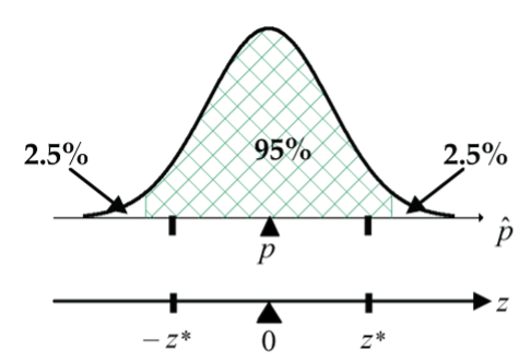
Acknowledging this variability in $\hat{p}$ , it seems unwise to put all our money on the exact value of 85%. Rather, we should estimate the population percentage $p$ with an interval of possible percentages that is likely to capture $p$ . We can use the 68–95–99.7 rule (empirical rule) from Lesson 2.3 plus our newly acquired knowledge of the sampling distribution of $\hat{p}$ from Lesson 3.1 to construct such an interval.

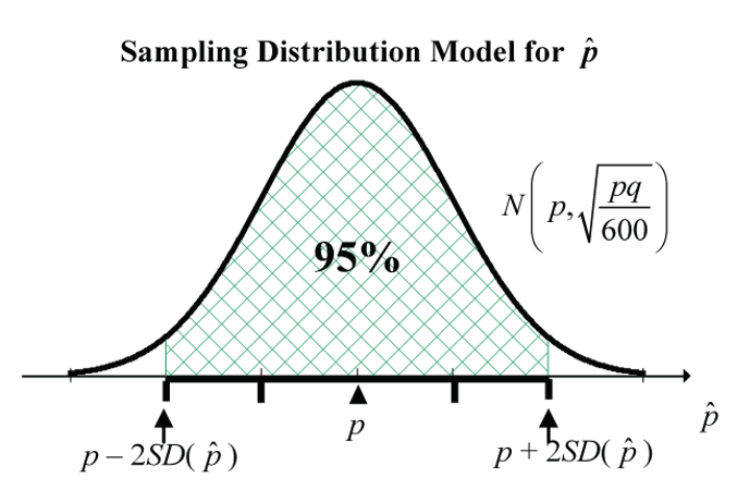
**Figure 1:** A sampling distribution model shows 95% confidence interval for a proportion

The sampling distribution says that about 95% of the potential values of $\hat{p}$ will be within two standard deviations of $p$ . Recall that the standard deviation of $\hat{p}$ is the standard error of $\hat{p}$ , $SE(\hat{p})=\sqrt{\dfrac{p(1-p)}{n}}=\sqrt{\dfrac{pq}{n}}$ , where $q=1-p$ .

We approximate the unknown $p$ by its sample estimate $\hat{p}$ . So, “two standard deviations” is $2\sqrt{\dfrac{pq}{n}} \approx 2\sqrt{\dfrac{\hat{p}\hat{q}}{n}} = 2\sqrt{\dfrac{0.85\times0.15}{600}} = 0.029 = 2.9\%$ .

So, 95% of the potential values of $\hat{p}$ will be within $2.9\%$ of the unknown $p$ . Since the Synovate poll referenced by Hume (2006) resulted in $\hat{p} = 85\%$ , and $85\%-2.9\% = 82.1\%$ and $85\%+2.9\% = 87.9\%$ , we can conclude that the interval from $82.1\%$ to $87.9\%$ likely captures (or contains) $p$ .

This interval is an approximate 95% confidence interval for proportion $p$ . To interpret the interval, we can say that we are 95% confident that the percentage of all GVRD residents supporting the expansion is between 82.1% and 87.9%.

Confidence Interval for a Population Proportion

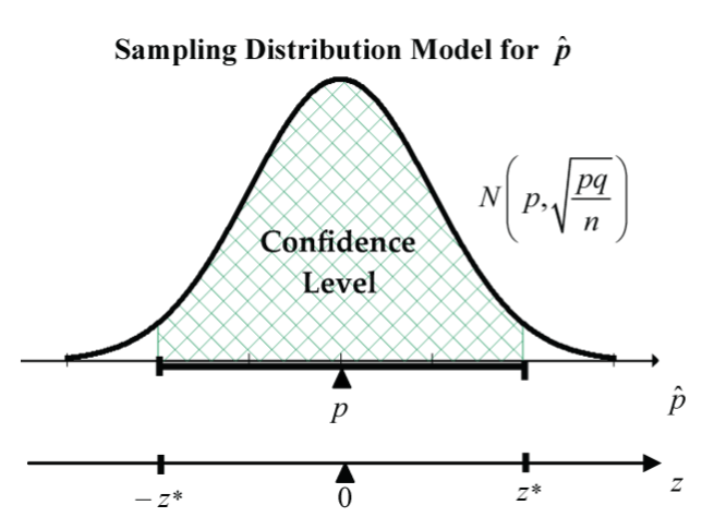
We just constructed an approximate 95% confidence interval for a population proportion. While 95% is a commonly-used confidence level, we could set the confidence level at any percentage between 0% and 100%. The following experiment is the general set-up for constructing a confidence interval for a proportion.

Experimental Situation

One categorical population with an unknown proportion (or percentage) $p$ .

Sampling a proportion — **Figure 2:** A sample estimate of a population is the sample proportion

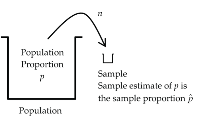
Objective

Based on the results of a random sample of $n$ observations from this population, construct a confidence interval for the unknown proportion $p$ .

Assumptions

Independence: The individual responses in the sample are independent of each other.
Random: The sample is random.
Success/Failure Condition: $n\hat{p} \ge 10$ and $n\hat{q} \ge 10$ .
10% Condition: The sample size $n$ is no more than 10% of the population size.

Confidence Interval Construction

The general form for a confidence interval for a proportion $p$ is $\hat{p} \pm z^* \times SE(\hat{p}) \approx \hat{p} \pm z^* \times \sqrt{\dfrac{\hat{p}\hat{q}}{n}}$ , where $z^*$ is the critical value z-score from the standard normal distribution corresponding to the specified confidence level.

The quantity $z^* \times SE(\hat{p})$ is called the margin of error of $\hat{p}$ , so the confidence interval can also be expressed as $\hat{p} \pm ME(\hat{p})$ , where the margin of error is $ME(\hat{p}) = z^* \times SE(\hat{p})$ .

Terminology

The standard error of $\hat{p}$ is the standard deviation of $\hat{p}$ based on its sampling distribution, $SE(\hat{p}) = \sqrt{\dfrac{pq}{n}}$ , which we estimate by $\sqrt{\dfrac{\hat{p}\hat{q}}{n}}$ .

The margin of error of $\hat{p}$ is the amount added to or subtracted from the point estimate, $\hat{p}$ , in the construction of a confidence interval for the population proportion, $p$ . It is calculated by multiplying a percentile from the normal distribution ( $z^*$ ) by the standard error of the point estimate, $SE(\hat{p})$ , i.e., $ME(\hat{p}) = z^* \times SE(\hat{p})$ .

Example: Confidence Interval for a Proportion

For the next example, first consider this excerpt of a news article (Bohn, 2006) published by The Vancouver Sun.

Most Believe Afghan Mission Not Working: Poll

By Glen Bohn (2006). Adapted from The Vancouver Sun.

As with other recent public opinion polls about the three-year-old deployment, the random sample of 550 B.C. adults underlines how divided voters are about the merits of keeping Canadian soldiers in Asia. (…) A slim 53-per-cent majority of those surveyed say they support the use of Canada’s troops for security and combat efforts against the Taliban in Afghanistan….

Construct a 90% and 95% confidence interval for the proportion of BC adults that supported the use of Canada’s troops against the Taliban in Afghanistan.

Condition Check

The assumptions required for the confidence interval calculation impose conditions on this data set. Are these conditions plausible?

Independence: Yes, individuals likely responded independently in this opinion poll.
Random: Yes, a random sample was taken.
Success/Failure Condition: Yes, $n\hat{p} = 550(0.53) = 291.5 \ge 10$ and $n\hat{q} = 550(0.47) = 258.5 \ge 10$ .
10% Condition: Yes, $n = 550$ is certainly less than 10% of the BC adult population.

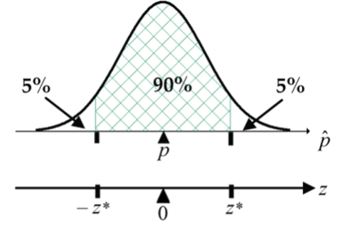
90% CI for $p$

In R, the code, qnorm(0.95, mean = 0, sd = 1) returns the critical z-score of 1.645, which has an area of 0.95 to the left and 0.05 to the right. You should be able to see from the diagram (Fig. 5) that the critical z-score of –1.645 has an area of 0.05 to the left and 0.95 to the right. Thus, the critical z-scores of –1.645 and 1.645 have an area of 0.90 in between.

**Figure 4:** A sampling distribution model shows 90% confidence interval for a proportion

$ME(\hat{p}) = z^* \times \sqrt{\dfrac{\hat{p}\hat{q}}{n}} = 1.645 \times \sqrt{\dfrac{0.53 \times 0.47}{550}} = 0.035 = 3.5\%$ .

90% CI for $p$ : $53\% \pm 3.5\%$ or (49.5%, 56.5%).

Interpretation: We are 90% confident that between 49.5% and 56.5% of adults in BC supported the use of Canada’s troops against the Taliban in Afghanistan.

95% CI for $p$

In R, the code, qnorm(0.975, mean = 0, sd = 1) returns the critical z-score of 1.96, which has an area of 0.975 to the left and 0.025 to the right. You should be able to see from the diagram (Fig. 6) that the critical z-score of –1.96 has an area of 0.025 to the left and 0.975 to the right. Thus, the critical z-scores of –1.96 and 1.96 have an area of 0.95 in between.

$ME(\hat{p}) = z^* \times \sqrt{\dfrac{\hat{p}\hat{q}}{n}} = 1.96 \times \sqrt{\dfrac{0.53 \times 0.47}{550}} = 0.042 = 4.2\%$ .

95% CI for $p$ : $53\% \pm 4.2\%$ or (48.8%, 57.2%).

Interpretation: We are 95% confident that between 48.8% and 57.2% of adults in BC supported the use of Canada’s troops against the Taliban in Afghanistan.

When you increase the confidence level from 90% to 95%, the price you pay for greater confidence is a wider interval! The 68–95–99.7 rule gives us $z^* = 2$ , which is just a rounded version of the more accurate value of $z^* = 1.96$ for 95% confidence.

Interpreting a Confidence Interval for a Proportion

Usually, constructing a confidence interval for a proportion is fairly straightforward, but correctly interpreting the interval can be tricky, particularly in the use of the word “confidence” (correct) vs “probability” (incorrect). The following simulation will provide us with greater insight into the correct interpretation of a confidence interval.

Imagine we have taken a random sample from a population in which $p = 0.5$ and we calculated the sample proportion to be 0.42 and a 95% confidence interval for $p$ to be from 0.32 to 0.52. Now imagine taking another random sample, but this time getting a sample proportion of 0.51 and a 95% confidence interval for $p$ going from 0.41 to 0.61.

Then let’s keep going. Figure 6 illustrates what the first seven samples might look like:

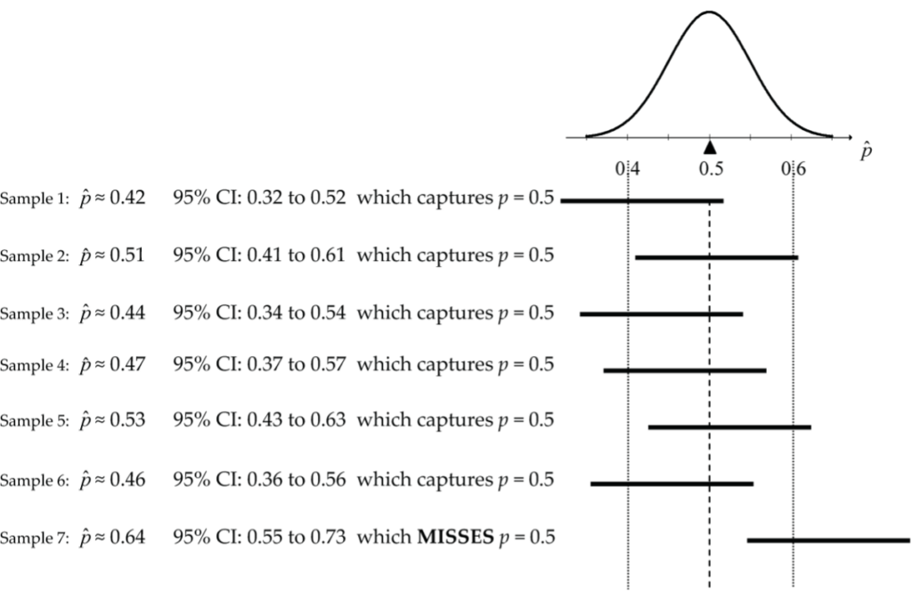
**Figure 6:** Confidence interval interpretation

If we were to continue this process of generating 95% confidence intervals, we know that in the long run 95% of them will capture $p$ , and that’s the sense in which we are “95% confident” in any particular CI. However, it is wrong to say that any particular CI has a 95% probability of capturing $p$ . Why? Nothing is random once the sample has actually been taken. For example, the probability that the first CI from 0.32 to 0.52 captures $p = 0.5$ is 100% (not 95%), and the last CI of 0.55 to 0.73 has 0% probability of capturing $p = 0.5$ .

When interpreting a 95% confidence interval, we say: “We are 95% confident that …” not “There is a 95% probability that ….”

References

Bohn, G. (2006, November 11). Most believe Afghan mission not working: poll. The Vancouver Sun [Excerpt]. https://advance.lexis.com/api/document?collection=news&id=urn:contentItem:4M9X-SPX0-TWD4-02G1-00000-00&context=1516831

Hume, M, (2006, November 9). A whale of support for aquarium expansion. The Globe and Mail [Excerpt]. https://www.theglobeandmail.com/news/national/a-whale-of-support-for-aquarium-expansion/article4112688/

License

Icon for the Creative Commons Attribution-NonCommercial-ShareAlike 4.0 International License

Introduction to Probability and Statistics Copyright © 2023 by Thompson Rivers University is licensed under a Creative Commons Attribution-NonCommercial-ShareAlike 4.0 International License, except where otherwise noted.