Lesson 1.3: Summarizing Numerical Data
Supplementary Notes 1.3
Summarizing Numerical Data
Histograms
Consider constructing a histogram from the following numerical data frequency table:
| Mother’s Age (years) | Number of Live Births |
| 10–14 | 4 |
| 15–19 | 1,421 |
| 20–24 | 6,101 |
| 25–29 | 11,032 |
| 30–34 | 13,129 |
| 35–39 | 7,062 |
| 40–44 | 1,483 |
| 45–49 | 85 |
| Total | 40,317 |
First let’s talk about the data:
- Who? Women giving live birth.
- What? Age of the women (the numerical variable)
- Where? British Columbia
- When? A given year
- How? The data was recorded by BC Ministry of Health (Vital Statistics Agency), via BC Data Catalogue: https://www2.gov.bc.ca/gov/content/data/bc-data-catalogue.
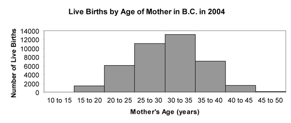
In this example, the frequency table giving the distribution of the mother’s age is already built for us. The most appropriate graphical representation of this frequency table is a histogram with the age categories on the horizontal axis and the frequencies (or percentage frequency) on the vertical axis:
Now, consider constructing a histogram from “raw” data. To draw a histogram from raw numerical data requires that we first construct a frequency table for the data. For large data sets, this can be a tedious task to do by hand, and it is usually done on a computer. No matter whether this task is done by hand or a computer, the basic steps are the same.
Let’s go through the steps of building a frequency table for the weights of players on the Vancouver Canucks hockey team in the 2013–2014 season.
| Name | Weight |
|---|---|
| Andrew Alberts | 218 lbs |
| Eddie Lack | 187 lbs |
| Kevin Bieksa | 198 lbs |
| Roberto Luongo | 217 lbs |
| David Booth | 212 lbs |
| Brad Richardson | 197 lbs |
| Alexandre Burrows | 188 lbs |
| Mike Santorelli | 189 lbs |
| Zac Dalpe | 195 lbs |
| Jordan Schroeder | 175 lbs |
| Alexander Edler | 215 lbs |
| Daniel Sedin | 187 lbs |
| Jason Garrison | 218 lbs |
| Henrik Sedin | 188 lbs |
| Dan Hamhuis | 209 lbs |
| Tom Sestito | 228 lbs |
| Jannik Hansen | 195 lbs |
| Ryan Stanton | 196 lbs |
| Chris Higgins | 205 lbs |
| Christopher Tanev | 185 lbs |
| Nicklas Jensen | 202 lbs |
| Dale Weise | 210 lbs |
| Zack Kassian | 214 lbs |
| Jeremy Welsh | 210 lbs |
| Ryan Kesler | 202 lbs |
- Locate the smallest (175 lbs) and largest (228 lbs) data values.
- Decide on a “bin” (class interval) width for your frequency table. There is no hard and fast rule for making this decision, but as a rule of thumb, choose a bin width that results in 5 (small data set) to 20 (large data set) bins for your data. With the small size of the Vancouver Canucks players’ weight data set, we want about 6 bins; so let’s choose a width of about (228 – 175) / 6 = 8.83 lbs. Make sure that you choose a “friendly” (i.e., easy-to-interpret) number for the bin width. In this case, let’s use a bin width of 10 lbs. We could use a bin width of 9 lbs, but when rounding to a “friendly” number, round up (otherwise, you might not cover all the data values). Often, a computer program will ask you what bin width you want.
- Choose a starting point for the first bin. The starting point could be the smallest data value or some “friendly” or meaningful number somewhat smaller than the smallest value. Let’s use 175 lbs as the starting value for the first bin.
- Build the bins using an “up to but not including” convention to avoid ambiguity of where a data value should be placed that falls right on a bin boundary.
| Canuck Weights (lbs) | Frequency |
| 175–184 | 1 |
| 185–194 | 6 |
| 195–204 | 7 |
| 205–214 | 6 |
| 215–224 | 4 |
| 225–234 | 1 |
| Sum of Frequencies | 25 |
Classes must not overlap. If you use classes such as 175–185, 185–195, 195–205, etc., you must indicate where the end points belong. Communicate this in a note, such as: Upper limit is not included in the class.
It is possible to end up with a different number of bins than you started with, and this is okay. This is due to rounding to a “friendly” number.
- Finally, we can draw the histogram corresponding to our frequency table.
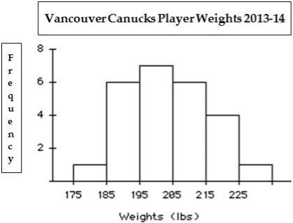
Figure 2: Histogram of Vancouver Canucks players’ weight, 2013-2014. Upper limit is not included in the class. [Long Description]
Interpreting or “Reading” a Histogram
Being able to interpret or “read” a histogram is the most important part of the process. Let’s read the histogram for the Vancouver Canucks players’ weights.
Shape: Visualize putting a mirror across the middle of the histogram perpendicular to the horizontal axis. Does the right side of the histogram look more or less like the left? If so, we call the histogram symmetric. The Vancouver Canucks players’ weight histogram (Fig. 2) is roughly symmetric. If a histogram is not symmetric, it is said to be asymmetric. If it has a drawn-out “tail” to the right, we say the histogram is skewed right. If the tail is drawn-out to the left, the histogram is skewed left.
Centre: Approximately where is the histogram centred? We will be much more precise in Unit 2 as to how we define the centre. For now, it is just an estimate of a typical middle value, like 200 lbs for the Canucks players’ weights histogram.
Spread: Again, we will define this concept much more carefully in Unit 2. The weights in the Canuck data set go from 175 lbs to 228 lbs, which is a range of 228 − 175 = 53 lbs.
Clustering: Does the data tend to cluster or concentrate in one (or more) places? Most of the Canucks players’ weights cluster in the 195 lbs to 205 lbs interval.
Gaps: If there are intervals with no measurements, then there will be a gap between the histogram bars. Gaps should be noted. The Canucks player data has no gaps.
Outliers: For now, an outlier is just any measurement that stands unusually above or below the others. Here, there is no obvious outlier.
Interpreting the Shape of a Histogram
The main purpose of a histogram is to display the frequency distribution of a numerical variable. The sketches below show some of the more common shapes for histograms, and they give examples of variables that likely have the corresponding shape.
- Symmetric, “bell” shaped, e.g., birth weights of full-term babies. Why? Birth weights of full-term babies tend to cluster around 3.4 kg with an approximate symmetric distribution of weights below and above 3.4 kg.

- Symmetric, uniform shaped, e.g., time of day an earthquake hits. Why? Each time interval throughout the day is equally likely for an earthquake.
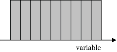
Figure 4: Symmetric, uniform shaped histogram [Long Description] - Asymmetric, skewed to the left, e.g., age of a person at death. Why? Deaths cluster in late-60s to late-80s with relatively fewer deaths in the younger years.
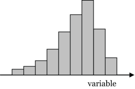
Figure 5: Asymmetric histogram skewed to the left [Long Description] - Asymmetric, skewed to the right, e.g., age at first marriage. Why? First marriage ages cluster in the 20s to early 30s, then the number of first marriages tails-off in later ages.
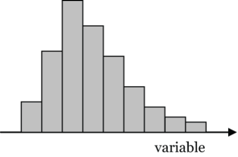
Figure 6: Asymmetric histogram skewed to the right [Long Description]
Constructing a Stem-and-Leaf Display
The stem-and-leaf display is sometimes used as an alternative to the histogram for displaying the distribution of a small numerical data set. Essentially, the “stem” part corresponds to the bins (classes) of the histogram, and the “leaves” form the equivalent of the bars.
Consider the Vancouver Canucks players’ weights again. A convenient choice for the stem is:
- 17, which represents 170 lbs to 179 lbs
- 18, which represents 180 lbs to 189 lbs
- etc.
Let’s make a column for the stem (smallest at the top) and draw a vertical line to the right of the column. Then, let’s fill in the “leaves” with the individual player weights as follows:
Stem Leaves
17 | 5
18 | 5 7 7 8 8 9
19 | 5 5 6 7 8
20 | 2 2 5 9
21 | 0 0 2 4 5 7 8 8
22 | 8
Key: 17 | 5 = 175 lbs
Figure 7: Stem-and-leaf display is an alternative to a histogram.
Be sure to order the leaves, and always give the leaf unit or a key. As you can see, the stem-and-leaf display for the players’ weight is essentially a sideways histogram, but it has the advantage of actually showing the individual player weights.
For large numerical data sets, the stem-and-leaf display is not really a practical display.
Constructing a Dot Plot
The dot plot is another alternative to the histogram and stem-and-leaf display. The dot plot provides a quick and easy way to display the distribution of a small numerical data set where there are only a few different values with multiple frequencies.
For example, consider the following Vancouver Canucks players’ heights:
| Name | Height |
| Andrew Alberts | 6ʹ 5ʺ |
| Kevin Bieksa | 6ʹ 1ʺ |
| David Booth | 6ʹ 0ʺ |
| Alexandre Burrows | 6ʹ 1ʺ |
| Zac Dalpe | 6ʹ 1ʺ |
| Alexander Edler | 6ʹ 3ʺ |
| Jason Garrison | 6ʹ 2ʺ |
| Dan Hamhuis | 6ʹ 1ʺ |
| Jannik Hansen | 6ʹ 1ʺ |
| Chris Higgins | 6ʹ 0ʺ |
| Nicklas Jensen | 6ʹ 2ʺ |
| Zack Kassian | 6ʹ 3ʺ |
| Ryan Kesler | 6ʹ 2ʺ |
| Eddie Lack | 6ʹ 4ʺ |
| Roberto Luongo | 6ʹ 3ʺ |
| Brad Richardson | 6ʹ 0ʺ |
| Mike Santorelli | 6ʹ 0ʺ |
| Jordan Schroeder | 5ʹ 8ʺ |
| Daniel Sedin | 6ʹ 1ʺ |
| Henrik Sedin | 6ʹ 2ʺ |
| Tom Sestito | 6ʹ 5ʺ |
| Ryan Stanton | 6ʹ 2ʺ |
| Christopher Tanev | 6ʹ 2ʺ |
| Dale Weise | 6ʹ 2ʺ |
| Jeremy Welsh | 6ʹ 3ʺ |
To make a dot plot for the heights of the players, put the various values of the players’ heights on the vertical (or horizontal) axis, then put a dot to the right for each player that has that height.
| Heights (ft. in) | Dots |
|---|---|
| 5ʹ 8ʺ | |
| 5ʹ 9ʺ | |
| 5ʹ 10ʺ | |
| 5ʹ 11ʺ | |
| 6ʹ 0ʺ | |
| 6ʹ 1ʺ | |
| 6ʹ 2ʺ | |
| 6ʹ 3ʺ | |
| 6ʹ 4ʺ | |
| 6ʹ 5ʺ |
Figure 8: Dot plot of Vancouver Canucks players’ heights, 2013–2014 season
The dot plot shows that the players’ heights are unimodal and centred near 6ʹ 2ʺ. Jordan Schroeder’s height (5ʹ 8ʺ) appears to be an outlier.
The 5-Number Summary
The 5-number summary of a numerical data set consists of: the minimum, 1st quartile (Q1), median, 3rd quartile (Q3), and maximum.
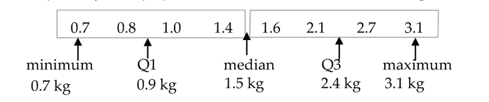
Example 1: Calculate the 5-number summary for a sample of 8 weight losses (kg) for people on a diet:
2.1 3.1 1.4 0.8 1.0 2.7 0.7 1.6
Important first step: put the numbers in order, smallest to largest.
0.7 0.8 1.0 1.4 1.6 2.1 2.7 3.1
Minimum = 0.7 kg
Q1 is calculated as the median of the bottom half of the measurements. Q1 = 0.9kg
For 8 ordered measurements, the median is the mean of the 4th and 5th measurements. Median = 1.5 kg
Q3 is calculated as the median of the top half of the measurements. Q3 = 2.4kg
Maximum = 3.1 kg
.
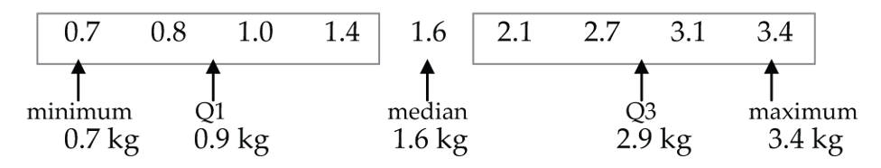
Example 2: Calculate the 5-number summary for a sample of 9 weight losses (kg) for people on a diet:
2.1 3.1 1.4 0.8 1.0 2.7 0.7 1.6 3.4
Important first step: put the numbers in order, smallest to largest.
0.7 0.8 1.0 1.4 1.6 2.1 2.7 3.1 3.4
If we exclude the median from the bottom half of the measurements, then Q1 is 0.9kg.
For 9 ordered measurements, the median is the 5th measurement, 1.6.
If we exclude the median from the top half the the measurements, then Q3 is 2.9kg.
Alternative method for calculating Q1 and Q3 when the sample size, n, is odd:
A simple rule for finding quartiles is to find the median of each half of the data split by the median. When n is even, the data splits in half unambiguously. But when n is odd, we can exclude or include the median with each of the halves.
In the example above for n = 9, we excluded the median from each half. However, if we include the median in each half then Q1 = 1.0 kg and Q3 = 2.7 kg.
So which method is right for an odd number of measurements?
They both are! This is not a case of right and wrong; rather it is a situation where two slightly different methods for calculating the quartiles are both valid. Different computer software packages use different methods (and some allow you to choose from different methods).
For large data sets it won’t matter much, since the two methods will give very similar values for Q1 and Q3.
Constructing a Boxplot
The table below gives the weights of the Vancouver Canucks players in ascending order:
| Order (Statistic) | Name | Weight |
| 1 (Minimum) | Jordan Schroeder | 175 lbs |
| 2 | Christopher Tanev | 185 lbs |
| 3 | Daniel Sedin | 187 lbs |
| 4 | Eddie Lack | 187 lbs |
| 5 | Alexandre Burrows | 188 lbs |
| 6 | Henrik Sedin | 188 lbs |
| 7 (Q1) | Mike Santorelli | 189 lbs |
| 8 | Zac Dalpe | 195 lbs |
| 9 | Jannik Hansen | 195 lbs |
| 10 | Ryan Stanton | 196 lbs |
| 11 | Brad Richardson | 197 lbs |
| 12 | Kevin Bieksa | 198 lbs |
| 13 (Median) | Nicklas Jensen | 202 lbs |
| 14 | Ryan Kesler | 202 lbs |
| 15 | Chris Higgins | 205 lbs |
| 16 | Dan Hamhuis | 209 lbs |
| 17 | Dale Weise | 210 lbs |
| 18 | Jeremy Welsh | 210 lbs |
| 19 (Q3) | David Booth | 212 lbs |
| 20 | Zack Kassian | 214 lbs |
| 21 | Alexander Edler | 215 lbs |
| 22 | Roberto Luongo | 217 lbs |
| 23 | Jason Garrison | 218 lbs |
| 24 | Andrew Alberts | 218 lbs |
| 25 (Maximum) | Tom Sestito | 228 lbs |
-
- Calculate the 5-number summary. Here n = 25, so the median is the (25 + 1) / 2 = 13th measurement. Thus, the median = 202 lbs. If we include the median with each half of the data to find Q1 and Q3, then since there are 13 numbers on each side, the median of those numbers is the 7th measurement in each half. Thus, Q1 = 189 lbs and Q3 = 212 lbs.
- Draw a horizontal or a vertical axis to represent the player weights.
- Draw a “box” stretching from Q1 to Q3. Draw a line through the box at the median.
- Calculate the interquartile range (IQR): IQR = Q3 – Q1 = 212 – 189 = 23 lbs.
- Calculate the lower fence and upper fence. Lower = Q1 – 1.5(IQR) = 189 – 1.5(23) = 154.5 lbs. Upper = Q3 + 1.5(IQR) = 212 + 1.5(23) = 246.5 lbs.
- Check for outliers below lower fence and above upper fence. No outliers here.
- Draw “whiskers” up and down to the most extreme values inside the fences (here the min and max). If there were outliers, they would be marked as isolated points outside the fences.
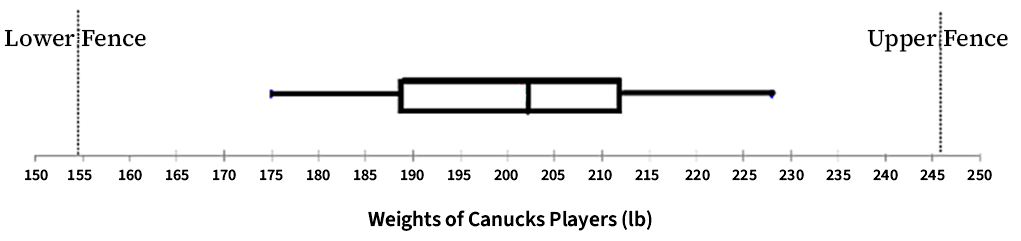
The distribution for the players’ weights is roughly symmetric, since the distribution of the data looks similar on both sides of the median.
Calculating the Mean and Standard Deviation
Mean:
![\[\begin{array}{l}\overline y = \dfrac{{\sum {y_i}}}{n}\\\text{where } \sum {y_i} \text{ is the Sum of the } {y}\text{'s and } {n} \text{ is the sample size} \end{array}\]](https://introprobabilityandstatistics.pressbooks.tru.ca/wp-content/ql-cache/quicklatex.com-d49ac78c1a22a15ccab06da485c7be5f_l3.png "Rendered by QuickLaTeX.com")
Sample of 5 weight losses (kg): 1.2 0.8 3.0 2.0 0.5
The individual measurements can be coded as y1, y2, y3, y4, y5.
1.2 (y1) 0.8(y2) 3.0(y3) 2.0(y4) 0.5(y5)
Calculate the mean weight loss:
![\[\begin{array}{l}\overline y = \dfrac{\text{total of the 5 weight losses}}{5}=\dfrac{7.5}{5}=1.5{\text{kg}}\]](https://introprobabilityandstatistics.pressbooks.tru.ca/wp-content/ql-cache/quicklatex.com-3fb1f364f517bfafddc0c33d27032d39_l3.png "Rendered by QuickLaTeX.com")
Next, calculate the standard deviation of the 5 weight losses, i.e., a value that will be used to represent a “typical” or “standard” deviation of the 5 weights from the mean of 1.5 kg.
Standard Deviation:
![\[s = \sqrt {\frac{{\sum {{{\left( {{y_i} - \overline y} \right)}^2}} }}{{n - 1}}} \]](https://introprobabilityandstatistics.pressbooks.tru.ca/wp-content/ql-cache/quicklatex.com-1c3e792e2210629b1497f08f8d1f506a_l3.png "Rendered by QuickLaTeX.com")
| Weights Losses (kg) |
Deviations from the Mean |
Squared Deviations |
| 1.2 | 1.2 – 1.5 = – 0.3 | (–0.3)2 = 0.09 |
| 0.8 | 0.8 – 1.5 = – 0.7 | (–0.7)2 = 0.49 |
| 3.0 | 3.0 – 1.5 = 1.5 | (1.5)2 = 2.25 |
| 2.0 | 2.0 – 1.5 = 0.5 | (0.5)2 = 0.25 |
| 0.5 | 0.5 – 1.5 = – 1.0 | (1.0)2 = 1.00 |
| Column totals |  |
 |
Standard deviation:  .
.
So, the standard (typical) deviation of the weight losses from the mean weight loss is about 1.01 kg.
Notice that the sum of the deviations from the mean equals 0. This will always be the case for every data set. It tells us that the mean is the balance point of the data set (because the sum of the negative deviations from the mean always balances the sum of the positive deviations from the mean).
Rounding Conventions:
- Round final answers for the mean and standard deviation to one more decimal place than the number of decimals used in the original data set.
- Do not round intermediate steps.
Comparing the Measures of the Centre
The mean and median are the most commonly used measures of the centre of a numerical data set. However, these two measures interpret the centre in very different ways, as the next example illustrates.
For the following two dot plots, each with 4 measurements, notice how the mean and the median behave as the largest value is increased from 4 (which is not an outlier) (Figure 12) to 8 (which is an outlier)(Figure 13).
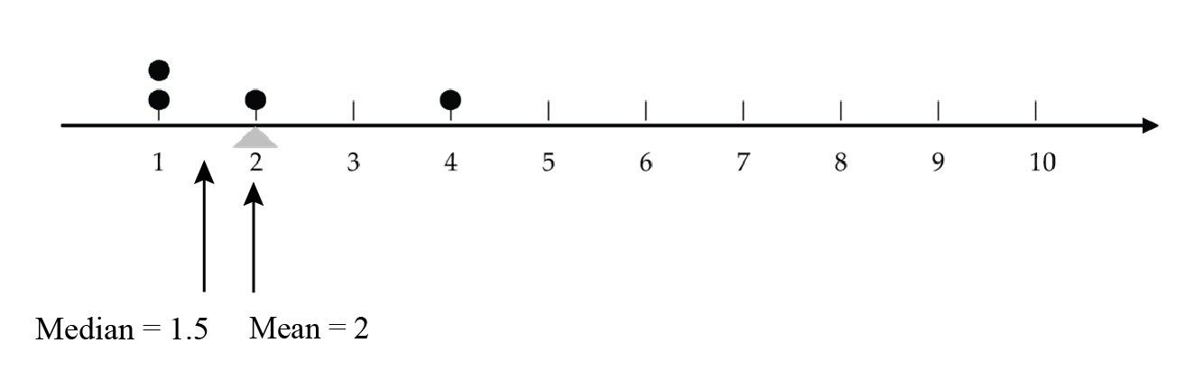
 and 2 is the balance point.
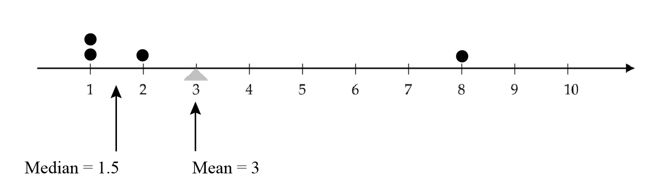
 and 3 is the balance point. Mean equals 3 since equation here and 3 is the balance point
The mean is “pulled” towards an outlier, since it measures the centre as a balance point. However, outliers do not affect the median since it measures the centre by cutting the data into a bottom half and a top half.
Comparing the Measures of Spread
Think of a measure of spread as an important companion measure to the measure of the centre. Although there is no hard and fast rule, the usual “centre-spread companions” are:
- mean and standard deviation (SD)
- median and interquartile range (IQR)
Why these pairings?
The SD is calculated by summing all of the squared deviations from the mean, dividing this sum by n − 1, and then taking the square root. Like the mean, it takes each and every data value into account in its calculation. Consequently, both the mean and the SD are sensitive to outliers. The SD represents a standard (or typical) deviation from the mean. It measures spread relative to the mean, so it fits as a companion measure to the mean.
On the other hand, both the median and IQR are based on the relative positioning of the measurements (as opposed to the actual values). Consequently, neither is sensitive to outliers. The IQR measures the spread in the sense that it gives you the distance spanned by the middle 50% of the data.
Choosing the Most Appropriate Measures of Centre and Spread
The mean and SD are well suited to symmetric, unimodal distributions that don’t have outliers. For the histogram below, the SD is just approximated showing what might be considered as a typical deviation of a data value from the mean.
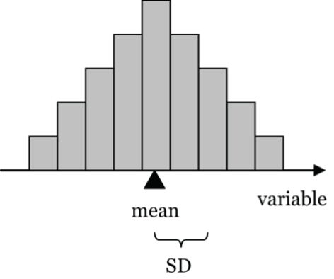
For example, birth weights of full-term babies tend to have this type of distribution with a mean of about 3.4 kg (7.5 lbs) and a SD of about 0.6 kg (1.32 lbs).
In Lesson 2.3, we will explore in much greater detail the importance of the SD for this type of distribution.
If the data is badly skewed (or has outliers), the median and IQR are more appropriate measures of the centre and spread.
The median divides the area of the histogram into two equal halves. For Figure 16, below, notice that there are 14 grid blocks below the median and 14 grid blocks above the median.
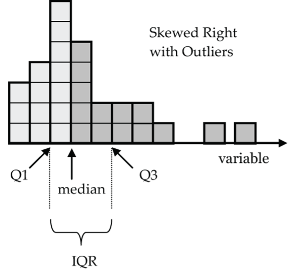
The first quartile Q1 has seven grid blocks below it and seven grid blocks between it and the median. Similarly, Q3 has seven grid blocks between it and the median and seven grid blocks above it. For a distribution like this one, the mean would be pulled up by the outliers to be a value greater than the median.
Can you think of an example of a distribution which has a shape like the one sketched? How about the salaries of the Vancouver Canucks (or any other professional sports team where usually there are a couple of very highly paid players with the bulk of the salaries clustering down at the median level)?
Long Descriptions
- Figure 1: Histogram of data from Table 1: Live Births by Age of Mother in B.C. The histogram has the categories along the x-axis and the Number of Live Births along the y-axis. The scale on the y-axis starts at 0 and goes up to 14000 by increments of 2000. No bar is shown for the 10 to 15 category as the value of 4 is too small to shown on this scale. The last category, 45-49, only shows a slightly darkened line. [Back to Figure 1]
- Figure 2: Histogram of the data from Table 3: Class Intervals (Bins) for Vancouver Canucks Hockey Players Weights (upper limit not included in the class). The histogram has the categories along the x-axis and the Frequency along the y-axis. The y-axis scale goes from 0 to 8 in increments of 2. A bar is displaying for each category. [Back to Figure 2]
- Figure 3: Symmetric “bell shaped” histogram graph showing the center of the graph has highest count for variable graphed, and then generally symmetrically decreasing away from that center value. Lower values for lower values of variable and then lower values for higher value of variable. [Back to Figure 3]
- Figure 4: Symmetric, uniform shaped histogram where every category of the variable has an equal count. The tops of the bars form a straight line. [Back to Figure 4]
- Figure 5: Asymmetric histogram skewed to the left where histogram peak is pushed to right towards higher values of variable so more categories with lower values. After peak the counts also drop off. “Skew” is the in the direction of the lower count categories. [Back to Figure 5]
- Figure 6: Asymmetric histogram skewed to the right where histogram peak is pushed to left towards lower values of variable so more categories with higher values. There is a very few categories before the peak and many after. “Skew” is the in the direction of the higher count categories. [Back to Figure 6]
- Figure 11: Boxplot showing Weight of Canucks Players in pounds in 5-pound increments is shown along the x-axis. A dashed vertical line is at 154.5 pounds and is labelled Lower Fence and a dashed vertical line is drawn at 246.5 and labelled Upper Fence. A thin rectangular box is drawn slightly above the x-axis with one end starting at Q1 (189 pounds) and the other ending at Q3 (212 pounds). Two “whiskers” extend from each side of the box towards the Fence lines. The whisker on the left goes to 175 pounds (minimum value) with a small vertical line marking the end of line. The whisker on the right goes to 228 pounds (maximum value) with a small vertical line marking the end of line. There is a vertical line across the box at 202 pounds. [Back to Figure 11]
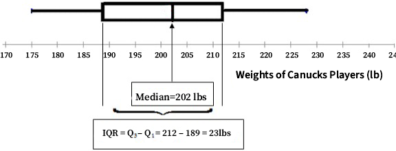
- Figure 14: Repeat of the Boxplot showing Weight of Canucks Players without Fences shown or labelled instead the vertical line at 202 pounds is labelled as median and it is shown that the ends of the box equal the IQR which is shown as equal to Q3 minus Q1 and for this example the values are 212 minus 189 equaling an IQR of 23 pounds. [Back to Figure 14]
- Figure 15: A generic Bell-shaped histogram showing that the Mean is at the peak of the histogram and that a Standard Deviation be a relatively small increment away from the mean. [Back to Figure 15]
- Figure 16: Histogram drawn with stacked blocks with 28 in total. The data is as follows, column 1 3 blocks, column 2 4 blocks, column 3 7 blocks, column 4 6 blocks, column 5 2 blocks, column 6 2 blocks, column 7 2 blocks, column 1 1 block, column 8 no blocks, then 2 single blocks spaced out further to right along axis. The median is labelled and occurs between column 3 and column 4, the IQR is shown with Q1 being between columns 2 and 3 while Q3 is being column 5 and 6. [Back to Figure 16]
References
BC Ministry of Health. (n.d.). Live births by age of mother in a given year [Data table]. https://www2.gov.bc.ca/gov/content/data/bc-data-catalogue
- Note. Data from BC Ministry of Health (n.d.) ↵
