Lesson 2.1: Probabilities of Events
Supplementary Notes 2.1
Basic Probability Concepts
In Lesson 1.2, we encountered several examples from journal abstracts where the sample results were judged to be statistically significant. In a very general sense, this means that the observed treatment differences are so large or unusual that they can’t be attributed to naturally occurring subject-to-subject variation. But how do statisticians measure “unusualness?” That’s where probability comes in. Probability is used to judge the unusualness of observed sample results.
Example
Here’s an example to illustrate the type of probabilistic thinking that statisticians use. At this point, don’t worry at all about how you actually calculate the probabilities to measure the unusualness. Rather, focus on the type of probabilistic thinking needed to reach the conclusion.
Suppose for a particular disease the standard drug in use has a cure rate of 50%. A new drug is tested on a random sample of 100 patients. Would you conclude that the new drug is more effective than the standard if:
- 51 of the 100 were cured?
Let’s think like a statistician! Suppose that the new drug really wasn’t any better than the standard, so it too had a cure rate of only 50%. Under this 50% cure model, is it unusual for a sample of 100 to produce 51 cures? Not at all. In this case, we would judge our sample results to be not statistically significant. The sample evidence is not strong enough for us to conclude (infer) that the new drug is more effective.
- 91 of the 100 were cured?
Hopefully, your intuition tells you that 91 cures out of 100 is a very unusual outcome under the 50% cure model. Consequently, we would judge our sample results to be statistically significant. The sample evidence is strong enough for us to conclude (infer) that the new drug is more effective.
- 58 of the 100 were cured?
This is a “grey zone”! This one is a tough call since 58 cures out of 100 certainly suggests that the new drug may have a higher cure rate than 50%, but how unusual is 58 cures if the true cure rate is still only 50%? Imagine flipping a coin 100 times. Would you be shocked if you got 58 heads and 42 tails? Unlike in scenario 2, our intuition about the unusualness of a grey zone result like 58 cures lets us down. We need some technical help in calculating probabilities to make this judgment about unusualness.
Technical help in calculating probabilities is on the horizon, so please read on!
What Is Probability?
Probabilities pop-up in daily life in a wide variety of contexts:
- The forecast shows a 60% chance of rain tomorrow.
- There is a 1 in 14 million chance that you win the “big one” in the Lotto 6/49.
- It is 50:50 that a single coin toss comes-up heads.
But how is probability defined? Probability is a very abstract idea, so it is a little tricky to pin it down with a single, nice, catch-all definition.
Probabilities for Repeatable Random Phenomena
Lottery draws and coin tosses are examples of random phenomena. A random phenomenon is any procedure that results in one of a number of known outcomes that can’t be predicted in advance.
For each outcome (e) of a random phenomenon, we define the probability of e to be the long-run relative frequency of e.
Symbolically:  in the long-run.
For example, flip a coin once:
- Probability of a head = P(head) = 1/2
- P(tail) = 1/2
This does not mean that if we flip the coin twice, we’ll get one head and one tail. Rather, it means that if we visualize flipping the coin over and over (forever!), the fraction of heads and the fraction of tails will each stabilize at 1/2. Long-run relative frequency is a very abstract mathematical concept that is easy to visualize for some random phenomena (like coin flips), but it is much tougher to visualize for more complicated phenomena.
For example, consider a spinner with a quarter of the circle shaded grey:

Spin the pointer once:
- P(grey) = 1/4
- P(white) = 3/4
The grey portion represents 1/4 of the full circle, so in the long-run the pointer will land in the grey area 1/4 of the time.
Personal Probabilities
When a weather forecaster gives 60% chance of rain for tomorrow, they are giving a probability that certainly does not fit the long-run relative frequency definition of probability, since tomorrow is NOT a repeatable random phenomenon. So, what does the 60% chance of rain mean? It is simply the weather forecaster’s (or the weather office’s) informed assessment of the likelihood of rain tomorrow. This is called a subjective or personal probability, and although it does not fit the same definition as that for repeatable random phenomena, it follows the same basic rules governing all probabilities.
Basic Concepts of Probability
Sample Space
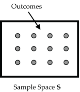
In probability applications, it is sometimes helpful to identify the entire collection of possible outcomes for a random phenomenon. This entire collection of possible outcomes is called the sample space and is designated by the letter S.
For example,
- Flip a coin: S = {head, tail}
- Roll a die: S = {1, 2, 3, 4, 5, 6}
Often, we use a Venn diagram to represent random phenomenon. In a Venn diagram, the sample space S is represented as an outer rectangle with the individual outcomes inside the rectangle.
“Rules of the Road” for Assigning Probabilities
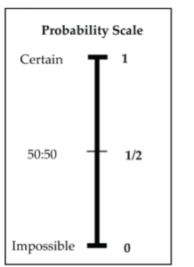
- The probability (P) of any outcome is always a number between 0 and 1.
- P(S) = 1 simply means that the probability (P) of something happening in the sample space (S) is 1.
- If an outcome is impossible, it has a probability of 0.
- If an outcome is certain to happen, it has a probability of 1.
Equally Likely Outcomes
In some probability applications, the individual outcomes in the sample space each have the same chance of occurring; i.e., the outcomes are equally likely.
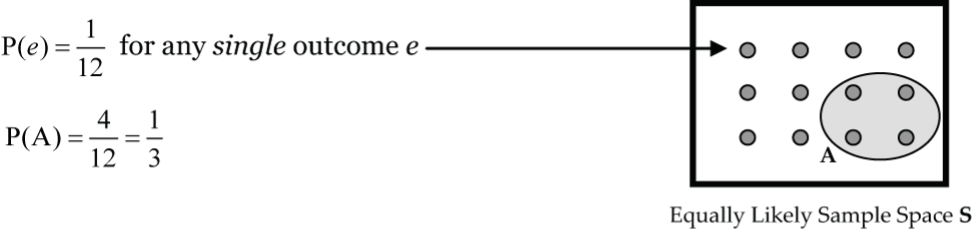
With a sample space of n equally likely outcomes, the probability of any one outcome is P(e) = 1/n. For an event A that consists of several equally likely outcomes, the probability of event A is P(A) = (# of outcomes in A)/n.
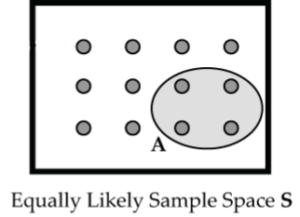
For example: In the sample space of 12 equally likely outcomes below (Figure 4):
![\[\begin{array}{c}\text{P}({e}) = \dfrac{1}{12}\text{ for any }single \text{ outcome } e\\ \text{P}(\text{A})&= \dfrac{4}{12} = \dfrac{1}{3}{array}\]](https://introprobabilityandstatistics.pressbooks.tru.ca/wp-content/ql-cache/quicklatex.com-34c18fdfe71257b3a0e03245c320ff88_l3.png "Rendered by QuickLaTeX.com")
P(e) = 1/12 for any single outcome e
P(A) = 4/12 = 1/3
Example: Card Deck with an Equally Likely Sample Space
A standard card deck has 52 cards that can be cross-classified by suit and type of card (as shown in Fig. 5),
| Diamond | Heart | Club | Spade |
| K | K | K | K |
| Q | Q | Q | Q |
| J | J | J | J |
| 10 | 10 | 10 | 10 |
| 9 | 9 | 9 | 9 |
| 8 | 8 | 8 | 8 |
| 7 | 7 | 7 | 7 |
| 6 | 6 | 6 | 6 |
| 5 | 5 | 5 | 5 |
| 4 | 4 | 4 | 4 |
| 3 | 3 | 3 | 3 |
| 2 | 2 | 2 | 2 |
| A | A | A | A |
| Red | Black | Red | Black |

If a card is drawn randomly from the deck, each of the 52 cards in the deck is equally likely; therefore, it has a 1/52 chance of being drawn. To find the probability of a more complicated event that consists of several cards, we simply determine how many cards there are in the event and then divide by 52.
For example, what is the probability that the randomly selected card is:
- The 3 of clubs? P(3 of clubs) = 1/52
- A club? P(Club) = 13/52 = 1/4
- An ace? P(Ace) = 4/52 = 1/13
- A face card (king, queen, or jack)? P(Face) = 12/52 = 3/13
- NOT a face card? P(NOT Face) = 40/52 = 10/13. Notice in this last example, P(NOT Face) = 1 – P(Face). This is an example of what is called in formal probability the complement rule because “NOT Face” is the complement of “Face.”
- A red ace? P(Red Ace) = 2/52 = 1/26
- NOT a red ace? P(NOT Red Ace) = 50/52 = 25/26
- A heart or a club? P(Heart or Club) = 26/52 = 1/2. Notice in this last example, P(Heart or Club) = P(Heart ) + P(Club). This is another example of a formal probability rule called the addition rule for disjoint (mutually exclusive) events. Although these formal rules are not really needed to answer questions for this card deck example, there are other probability applications where they are helpful. We will cover these formal probability rules next.
Basic Rules of Probability
Complement Rule
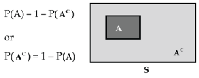
The probability of an event occurring is 1 minus the probability that it doesn’t occur. An event not occurring is denoted by “superscript C”; i.e., the complement of event A is denoted AC :
P(A) = 1 – P(AC) or P(AC) = 1 – P(A)

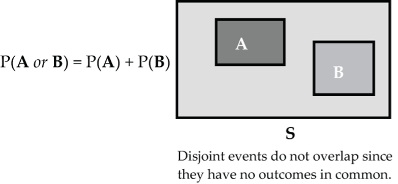
Addition Rule for Disjoint Events
Two events are called disjoint (mutually exclusive) if they have no outcomes in common. For two disjoint events, the probability of A or B is:
P(A or B) = P(A) + P(B)

Multiplication Rule for Independent Events
Two events are called independent if knowing that one occurs does not change the probability that the other event occurs. For two independent events, the probability of A and B is:
P(A and B) = P(A) • P(B)
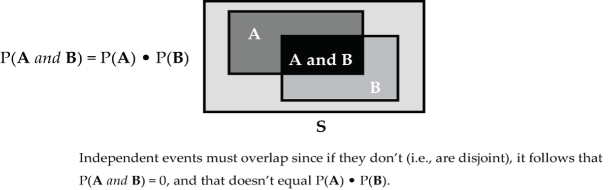
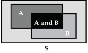
Independent events must overlap in a Venn diagram (see Fig. 8), since if they don’t (i.e., are disjoint), it follows that P(A and B) = 0, and that doesn’t equal P(A) • P(B).
Example
When the pointer of the spinner we considered in Figure 1 is spun twice, the chance that the first spin comes-up in the white region (W1) and the second spin in the grey region (G2) is:
P(W1 and G2) = P(W1) • P(G2)
P(W1 and G2) = 3/4 • 1/4 = 3/16
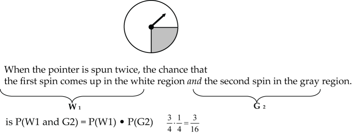
Here W1, G2 are clearly independent events since knowing the first spin comes-up white does not change the probability that the second spin comes -up grey.
Calculating Probabilities for Independent Events
Let’s consider some examples:
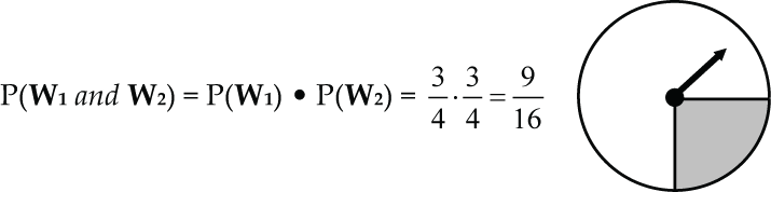
1. When the pointer in Figure 1 is spun twice, the chance that both spins come-up white is: P(W1 and W2) = P(W1) • P(W2) = 3/4 • 3/4 = 9/16
2. When the pointer (Fig. 1) is spun three times, the chance that all three spins come-up white is:
P(W1 and W2 and W3) = P(W1) • P(W2) • P(W3) = 3/4 • 3/4 • 3/4 = 27/64

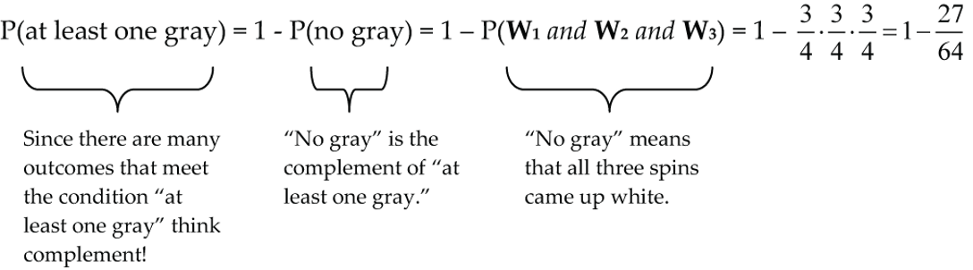
3. When the pointer (Fig. 1) is spun three times, the chance that at least one spin comes-up grey is:
P(at least one grey) = 1 – P(no grey)
P(at least one grey) = 1 – P(W1 and W2 and W3)
P(at least one grey) = 1 – 3/4 • 3/4 • 3/4 = 1 – 27/64 = 37/64
Now let’s try some examples using an exam. Let’s say: A multiple-choice test consists of four questions where each question has five possible answers, with one correct answer for each question. An ill-prepared student (not you of course) decides to guess randomly the answer to each question.
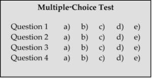
Find the chance that the student gets:
1. All four questions correct. Let’s explore this:
C1 = student gets first question correct, C2 = second question correct, etc.
P(C1) = 1/5 since only 1 of the 5 possible answers is correct, and the student is guessing randomly for each question. So, we get:
P(C1 and C2 and C3 and C4) = P(C1) • P(C2) • P(C3) • P(C4) = 1/5 • 1/5 • 1/5 • 1/5 = 1/625 = 0.0016 = 0.16%
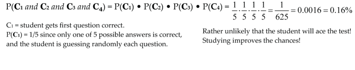
It is rather unlikely that a student who guesses random answers on a multiple-choice test will ace the test! Studying will improve the chances of passing a test!
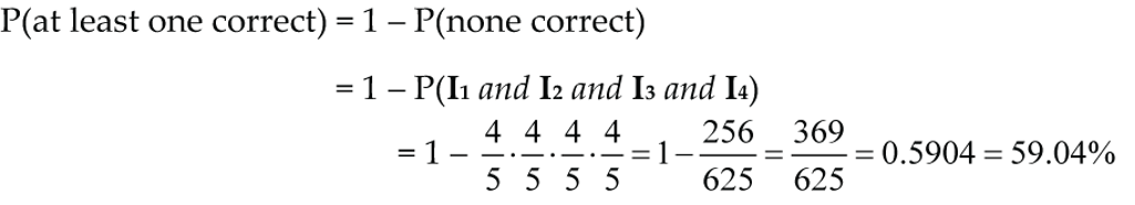
2. At least one question correct:
P(at least one correct) = 1 – P(none correct)
P(at least one correct) = 1 – P(I1 and I2 and I3 and I4)
P(at least one correct) = 1 – 4/5 • 4/5 • 4/5 • 4/5 = 1 – 256/625 = 369/625 = 0.5904 = 59.04%
General Addition Rule
The addition rule and multiplication rules we’ve considered so far only cover specific types of events:
- Addition Rule for Disjoint Events: P(A or B) = P(A) + P(B).
- Multiplication Rule for Independent Events: P(A and B) = P(A) • P(B).
Next, we extend the addition rule to cover in general any two events A, B. First a “warm-up” example that will set this up.
Example
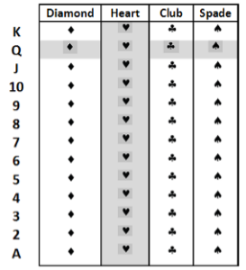
What is the probability that you get a queen or a heart when you randomly select one card from the card deck?
| Diamond | Heart | Club | Spade |
| K | K | K | K |
| Q | Q | Q | Q |
| J | J | J | J |
| 10 | 10 | 10 | 10 |
| 9 | 9 | 9 | 9 |
| 8 | 8 | 8 | 8 |
| 7 | 7 | 7 | 7 |
| 6 | 6 | 6 | 6 |
| 5 | 5 | 5 | 5 |
| 4 | 4 | 4 | 4 |
| 3 | 3 | 3 | 3 |
| 2 | 2 | 2 | 2 |
| A | A | A | A |
First, let’s be clear on the meaning of a queen or a heart. The randomly selected card could be any one of the 4 queens or any one of the 13 hearts. Notice that we are including the queen of hearts card, but we don’t want to count it twice. There are 16 cards in the event “queen or a heart” (shaded in Fig. 16). So, P(queen or heart) = 16/52.
But, can we calculate P(queen or heart) simply by adding P(queen) and P(heart)? Let’s try it: P(queen) + P(heart) = 5/52 + 13/52, which is not equal to P(queen or heart) since we just showed that was 16/52.
This shows that the addition rule for disjoint events doesn’t work here, and the reason is because the events “queen” and “heart” are not disjoint.
How could we modify this calculation so that it does give the correct answer 16/52?
P(queen or heart) = P(queen) + P(heart) – P(queen and heart) = 4/52 + 13/52 – 1/52 = 16/52.
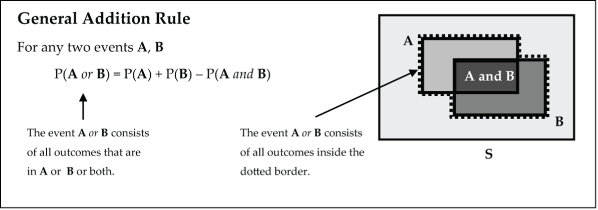
Now we’ve got it right! And we’ve set up the General Addition Rule: For any two events A, B the event A or B consists of all outcomes that are in A or B or both.
P(A or B) = P(A) + P(B) – P(A and B)
Example
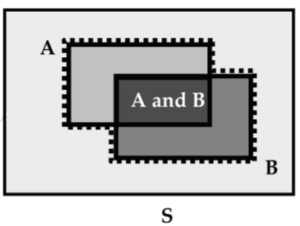
Wilma, a web design whiz, bids for work on two design projects. She feels that she has a 75% chance of getting the first project, a 45% chance of getting the second project, and a 25% chance of getting both projects.
1. What is the chance that she gets at least one of the two projects? Let A = {gets first project} and B = {gets second project}. Then the question asks for:
P(A or B) = P(A) + P(B) – P(A and B) = 0.75 + 0.45 – 0.25 = 0.95.
So Wilma has a 95% chance of getting at least one of the two projects.
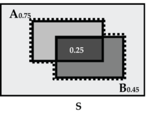
2. What is the chance that she gets only the first project? In the Venn diagram (Fig. 19), the event “only the first project” is the light gray part of event A that is outside of event B. It is symbolically given by A and BC. So, the question asks for:
P(A and BC) = P(A) – P(A and B) = 0.75 – 0.25 = 0.50
She has a 50% chance of getting only the first project.
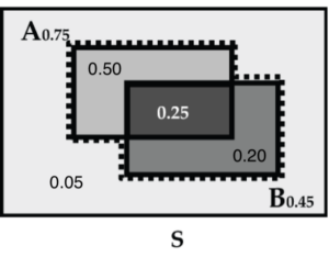
3. What is the chance that Wilma gets only the second project?
P(AC and B) = P(B) – P(A and B) = 0.45 – 0.25 = 0.20, so she has a 20% chance of getting only the second project.
4. What is the chance that she gets neither project?
P(AC and BC) = 1 – 0.50 – 0.25 – 0.20 = 0.05, so she has only a 5% chance of getting neither project.
