Supplementary Notes 2.3

Iain Pardoe

Lesson 2.3: The Normal Distribution

Supplementary Notes 2.3

The Normal Model

Introducing the Standard Deviation as a Ruler

Let’s start with an example: How unusual is a birthweight of 4,750 grams? Table 1 presents birth weight data for babies born in British Columbia in 2003.

Table 1 Birth Weight (Grams) for British Columbia, 2003
Birth Weight
(in Grams)	Total
<500	46
500–749	58
750–999	76
1,000–1,249	76
1,250–1,499	100
1,500–1,749	130
1,750–1,999	248
2,000–2,249	450
2,250–2,499	945
2,500–2,749	1,895
2,750–2,999	3,761
3,000–3,249	6,346
3,250–3,499	7,820
3,500–3,749	7,413
3,750–3,999	5,375
4,000–4,249	3,145
4,250–4,499	1,463
4,500–4,749	594
4,750–4,999	197
5,000–5,249	70
5,250–5,499	18
5,500+	17
Total	40,243
Source: (BC Ministry of Health, 2003)

Mean birth weight: 3,400 grams
Standard deviation: 600 grams

There are many ways of answering a question like this, but one of the most important ways in statistics is to use the standard deviation as a ruler to determine how many standard deviations the measurement is above or below the mean. Figure 1 uses the birth weight data (Table 1) in a histogram.

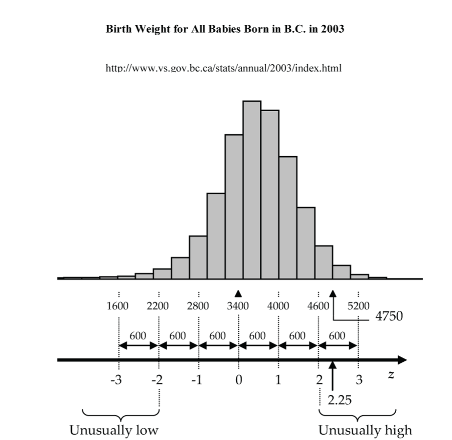
Birth weights histogram — **Figure 1:** Birth weight histogram for all babies born in BC in 2003. Data source: (BC Ministry of Health, 2003)

In standard deviation language (Z-score language), a birth weight of 4,750 grams is (4,750–3,400) / 600 = 2.25 SDs above the mean.

Z-score, $z = \dfrac{y-\overline{y}}{s}$ , where $y$ is the data value, $\overline{y}$ is the sample mean, and $s$ is the sample standard deviation (SD).

From the frequency table (Table 1), we can see that there are only 302 birth weights out of 40,243 (less than 1%) that are more than 4,750 grams (2.25 SDs) above the mean. As a rule, Z-scores of two or more are considered unusually high, and –2 or less unusually low.

Using Z-Scores to Compare Results

A very useful advantage of converting measurements to Z-scores is that it allows us to compare measurements that come from very different distributions. Using Z-scores we really can compare apples and oranges.

Here’s an example: Suppose a university wants to award a scholarship that is based equally on a student’s high school grade average and first-term college grade average. Which of the two students should get the scholarship?

Strategy

Table 2 provides grade point average data for Lisa and Kyle, and it tells the mean and SD for all students.

Table 2 High School and First-Term College Grade Averages
	High School Grade (%)	First-Term College GPA
Lisa	95.1	3.87
Kyle	90.3	4.12
Mean (all students)	78.4	2.85
SD (all students)	7.2	0.94

First, let’s convert the students’ grades into Z-scores (Table 3).

Table 3 Grades Converted to Z-Scores
	High School Z-score	First Term College Z-score
Lisa	(95.1 – 78.4) / 7.2 = 2.32	(3.87 – 2.85) / 0.94 = 1.09
Kyle	(90.3 – 78.4) / 7.2 = 1.65	(4.12 – 2.85) / 0.94 = 1.35

Next, we can add the Z-scores for each student (Table 4).

Table 4 Combined Z-Scores
	*Combined Z-scores*
Lisa	2.32 + 1.09 = 3.41
Kyle	1.65 + 1.35 = 3.00

Now, it’s clear that Lisa deserves the scholarship because she has the higher overall combined Z-score.

Introducing the Normal Model

In the previous birth weight example, we used the empirical distribution of a large sample to determine that less than 1% of the birth weights were greater than 4,750 grams (or equivalently, less than 1% of the Z-scores for this distribution were above 2.25).

But often we don’t have a large sample distribution to compare to, so how do we judge the unusualness of measurements and Z-scores?

**Figure 2:** Sample distribution unavailable

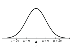
Answer: We create a model distribution (smoothed-out, idealized histogram) that we think will approximate the distribution of the measurements (see Fig. 3).

**Figure 3:** Normal curve in an idealized histogram shows model distribution

The normal model is the world’s most commonly-used model. (You’ll see why later in the course!)

Note: To distinguish models from data, we use the symbol µ (mu) for the mean of a model and σ (sigma) for the SD of a model.

The normal model is appropriate for variables (or data) that you expect to have a distribution that is unimodal, reasonably symmetric, and bell-shaped.

Which of the following variables do you think might follow (approximately) a normal model?

Weights of all 30-year-old males in Vancouver?

No. Heavier weights probably are distributed further out above the mean compared to the distribution of lighter weights below the mean. This distribution is likely skewed right.

Foot lengths of all adult females in Vancouver?

Yes. The normal model seems reasonable since foot lengths that are smaller than the mean likely distribute out in roughly the same symmetric way as longer foot lengths do above the mean.

The 68–95–99.7 Rule

The 68–95–99.7 rule (also called the empirical rule) makes use of the following facts about normal models:

Approximately 68% of the measurements are within one SD of the mean (Fig. 4).

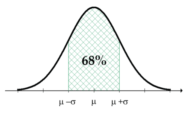
Figure 4: A normal curve has approximately 68% of measurements within one SD of the mean (µ)
Approximately 95% of the measurements are within two SDs of the mean (Fig. 5).

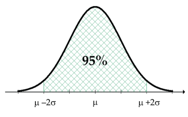
Figure 5: A normal curve has 95% of measurements within two SDs of the mean (µ)
Approximately 99.7% of the measurements are within three SDs of the mean (Fig 6).

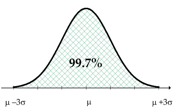
Figure 6: A normal curve has approximately 99.7% of measurements within three SDs of the mean (µ)

Applying the 68–95–99.7 Rule

Let’s assume that the foot length of adult females follows a normal model with a mean of 10 inches (25.4 cm) and an SD of 0.5 inches (1.27 cm). Use the model to determine the approximate percentage of foot lengths that are:

Between 9 and 11 inches (Fig 7).

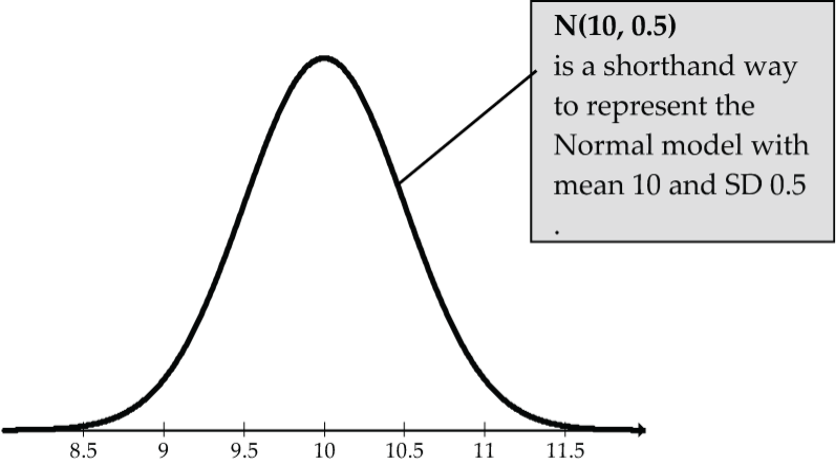
Figure 7: The normal curve N(10, 0.5), mean 10, SD 0.5

Notice that 9 inches is two SDs below the mean, and 11 is two SDs above the mean, so approximately 95% of the foot lengths are between 9 and 11 inches.
Greater than 11 inches (Fig. 8)

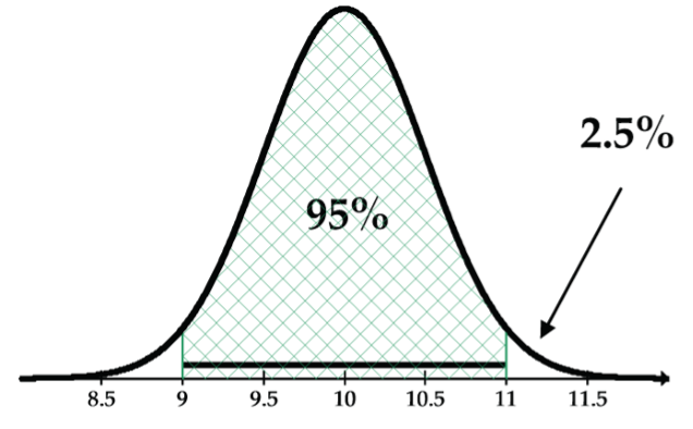
Figure 8: The normal curve N(10, 0.5), mean 10, SD 0.5, and an upper tail.

Well, if approximately 95% of the foot lengths are within two SDs of the mean, then approximately 5% are more than two SDs from the mean.
So, that means that approximately 5%/2 = 2.5% of the foot lengths are greater than 11 inches.
Less than 10.5 inches (Fig 9).

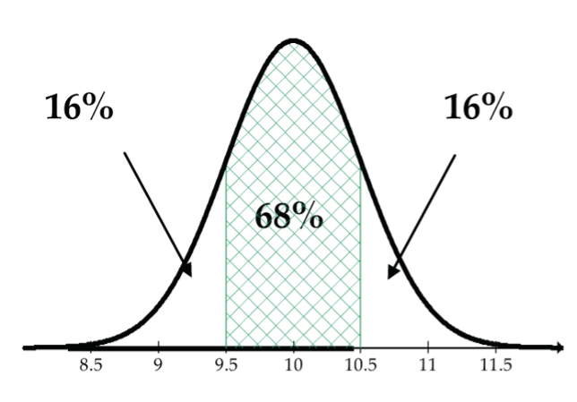
Figure 9: The normal curve N(10, 0.5), mean 10, SD 0.5, and a lower tail

10.5 inches is one SD above the mean, so approximately 68% of the foot lengths are between 9.5 and 10.5 inches. The remaining 32% is evenly split in the two tails. So, approximately 16% + 68% = 84% of the foot lengths are less than 10.5 inches.

Using Statistical Software to Find Normal Model Percentages: Part 1

For the N(10, 0.5) foot length normal model, we calculated percentages using the 68–95–99.7 rule. What do we do if we want to get percentages corresponding to foot lengths that don’t fall exactly one, two, or three SDs from the mean? For example, what percentage of the foot lengths is between 9.25 and 10.75 inches?

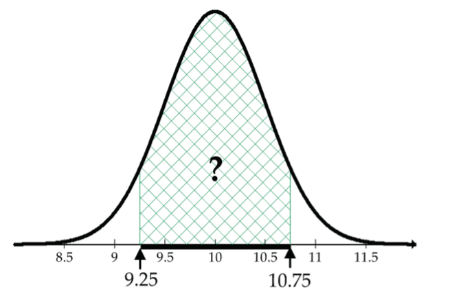
Normal curve, mean 10, sd 0.5, probability between 9.25 and 10.75 — **Figure 10:** A normal curve N(10, 0.5), mean 10, SD 0.5, to calculate probability between 9.25 and 10.75

In the good-old-days, this type of question would have been answered by first converting 9.25 and 10.75 to Z-scores (–1.5 and 1.5 respectively), then these Z-scores would have been looked-up in a table. OpenIntro Statistics goes through the table steps in Appendix C.1 (Diez et al., 2019) CC BY-SA 3.0.

Fortunately, statistical software makes it much easier to answer this type of question. In jamovi, click the plus button at the top right part of the screen, select jamovi library, and add the distrACTION module. Next, select Analyses > distrACTION > Normal Distribution, type “10” for the mean and “0.5” for the SD, select Compute probability, type “9.25” for x1, select “P(x1 $\le$ X $\le$ x2),” and type “10.75” for x2. You should see the resulting probability “0.866” and a normal curve with the shaded area between 9.25 and 10.75 corresponding to this probability.

Alternatively, click the plus button at the top right part of the screen, select jamovi library, and add the Rj - Editor to run R code inside jamovi module. Next, select Analyses > R > Rj Editor. Copy/paste the following code into the Rj Editor window: pnorm(10.75, mean=10, sd=0.5) - pnorm(9.25, mean=10, sd=0.5). If you run this code, jamovi returns the answer of 0.8664. This means that about 86.64% of the foot lengths are between 9.25 and 10.75 inches.

Note: To complete most of the assessments in this course, you’ll use statistical software to calculate normal model percentages rather than using the table method. However, understanding how the table method works will deepen your understanding of how to use the normal model. Also, you’ll need to understand the correspondence between Z-scores and percentiles in a normal probability table in order to answer some questions in the midterm and final exams. To self-assess your understanding, go through the textbook examples in Appendix C.1 using statistical software to confirm the percentages.

Example of Normal Model Percentages

Suppose that the fat content in 50-gram hamburger patties follows a normal model with a mean fat content of 12 grams and a SD of 1.2 grams.

What percentage of the hamburger patties has fat content between 11 and 13 grams?

pnorm(13, mean=12, sd=1.2) - pnorm(11, mean=12, sd=1.2)
= 0.5953

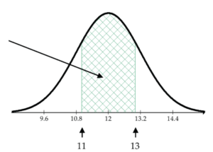
**Figure 11**: Normal curve, mean 12, SD 1.2, between 11 and 13 grams of fat

So, about 59.53% of the patties have fat content between 11 and 13 grams.

What percentage of the hamburger patties has fat content more than 14 grams?

1 - pnorm(14, mean=12, sd=1.2)
= 0.04779

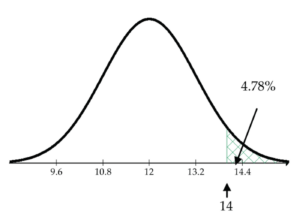
normal curve - mean 12, sd 1.2, more than 14 — **Figure 12**: Normal curve, mean 12, SD 1.2, more than 14 grams of fat

So, about 4.78% of the patties have more than 14 grams of fat content.

Using Statistical Software to Find Normal Model Percentages: Part 2

Statistical software can also be used to get percentages for the Z-score normal model that has a mean of 0 and a SD of 1. This special normal model is called a standard normal model and is abbreviated as N(0, 1). It is the N(0, 1) model that the tables in Appendix C.1 (Diez et al., 2019) CC BY-SA 3.0 give percentages for, but we will use statistical software.

To self-assess your understanding, you might want to compare the software values to those in the Appendix C.1 table. To help you, here are the relevant table entries for the three examples below:

Table 5 Z-Scores from Appendix C.1
z	1.75	2	2.25
P(Z ≤ z)	0.95994	0.97725	0.98778

For example, the probability a normal Z-score is less than or equal to 1.75 is 0.95994. Therefore, the probability a normal Z-score is greater than 1.75 is 1–0.95994 = 0.04006. Similarly, the probability a normal Z-score is less than –1.75 is 0.04006 (because the normal model is symmetric about 0). And the probability a normal Z-score is between –1.75 and 1.75 is 1–2(0.04006) = 0.91988.

For the standard normal model, what percent of the Z-scores are between –2 and 2?

pnorm(2) - pnorm(-2)
= 0.9545, which is approximately 95%. This is no surprise, as it is just as the 68–95–99.7 rule said it would be!

What percent of the Z-scores are less than –1.75?

standard normal curve - less than -1.75 — **Figure 13**: Standard normal curve, less than -1.75

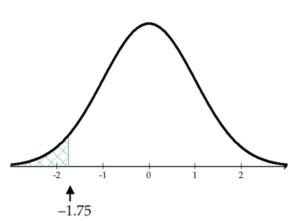
pnorm(-1.75)
= 0.04006
About 4.01% of the Z-scores are less than –1.75.

What percent of the Z-scores are greater than 2.25?

1 - pnorm(2.25)
= 0.01222

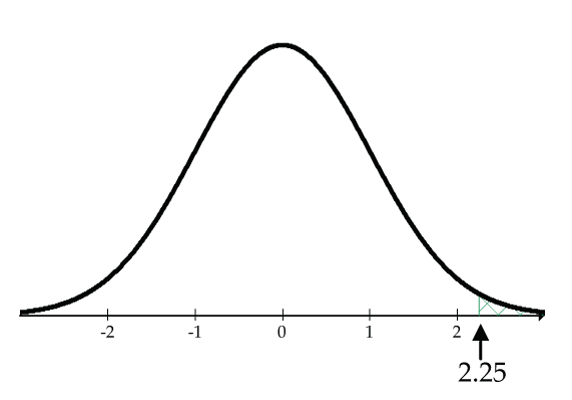
standard normal curve - greater than 2.25 — **Figure 14:** Standard normal curve, greater than 2.25

Only about 1.22% of the Z-scores are greater than 2.25. Consequently, a Z-score of 2.25 would be considered unusually high in the normal model.

Using Statistical Software to Find Normal Model Percentiles: Part 3

Reverse gear! Now we are going to use the normal model to get variable values along the axis that cut-off given percentages (areas under the curve).

normal curve - percentile — **Figure 15**: Given a percentile, the normal curve reveals the value of a variable that cuts-off the given area A.

Again, the OpenIntro Statistics textbook shows how to find these values using the table in Appendix C.1, but we’ll use statistical software because the calculations are far more direct.

Let’s again assume that the foot length of adult women follows a normal model with a mean of 10 inches and a SD of 0.5 inches. With this model, 25% of the foot lengths are less than which value?

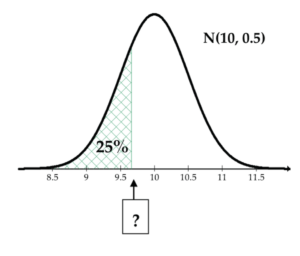
normal curve - mean 10, sd 0.5, 25th percentile — **Figure 16:** Normal curve N(10, 0.5) for adult women foot length, mean 10, SD 0.5, 25th percentile

In jamovi, select Analyses > distrACTION > Normal Distribution, type “10” for the mean and “0.5” for the SD, select Compute quantile(s), type “0.25” for p, and select “cumulative quantile.” You should see the resulting 25^th percentile “9.66” and a normal curve with the percentile marked. So, approximately 25% of the foot lengths are less than 9.66 inches.

Alternatively, select Analyses > R > Rj Editor and use the R code qnorm(A, mean, sd). Remember to express A as a decimal, not a percentage; i.e., qnorm(0.25, mean = 10, sd = 0.5). Run this code to return the answer 9.663.

With this model, 10% of the foot lengths are greater than which value?

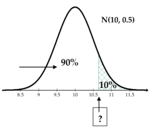
normal curve - mean 10, sd 0.5, 90th percentile — **Figure 17**: Normal curve N(10, 0.5) for adult women foot length, mean 10, SD 0.5, 90th percentile

Note that we must always enter the area to the left of the value that we are looking for (which is 0.9 in this case).
qnorm(0.9, mean = 10, sd = 0.5)
= 10.64.
Approximately 10% of the foot lengths are greater than 10.64 inches.

Using R to Find Normal Model Parameters

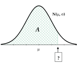
Now we’re ready to tackle a slightly more challenging application of normal models: How to find the value of the missing mean, μ, or standard deviation, σ (the parameters of the normal model).

For the normal model sketched in the Figure 18 diagram, find the value of the missing SD, σ.

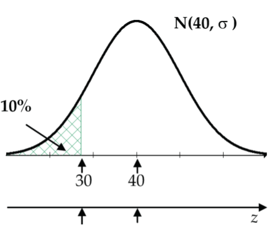
Figure 18: Normal curve to find SD

Strategy: Convert 30 to a Z-score: (30 – 40) / σ = Z.
Rearrange equation to σ = (30 – 40) / Z.
Calculate Z: qnorm(0.1) = –1.282.
So, σ = (30 – 40) / –1.282 = 7.800.
Check: pnorm(30, mean=40, sd=7.800) = 0.09991 ≅ 10% as given. It checks out!
r the normal model sketched in the Figure 19 diagram, find the value of the missing mean, μ.

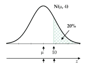
Figure 19: Normal curve to find mean

Strategy: Convert 10 to a Z-score: (10 – μ) / 4 = Z.
Rearrange equation to μ = 10 – 4Z.
Calculate Z: qnorm(0.8) = 0.8416.
So, μ = 10 – 4(0.8416) = 6.6336.
Check: 1 - pnorm(10, mean=6.6336, sd=4) = 0.2 = 20% as given. It checks out!

Using Statistical Software to Draw a Normal Probability Plot

How do we know if it is reasonable to assume a normal model for a particular variable or data set?

This is a tough question! If we have a large data set, we could check the reasonableness of assuming a normal model by drawing a histogram. If the histogram is unimodal, reasonably symmetric, and bell-shaped, then it is appropriate to assume a normal model.

Drawing a histogram requires judgement in constructing the bins, and unless we have a large data set it will be tricky to judge whether or not a normal model is appropriate.

There is a better type of graph specifically designed to judge the reasonableness of assuming a normal model. This graph is called a normal probability plot (or quantile-quantile plot or Q–Q plot), and it is built-in as one of the statistical plots in jamovi and R. The following example shows how to draw and how to interpret a normal probability plot.

Example

Is it reasonable to assume a normal model for the following sample of 20 test scores (Table 6)?

Table 6 Twenty Test Scores
Test Scores
62	35	95	86	66
91	49	73	84	89
83	62	88	62	54
46	81	66	68	60

Download the test [CSV file] data, and open it in jamovi.

Then select Analyses > Exploration > Descriptives, move test into the Variables box, and select Plots > Q-Q Plots: jamovi draws a normal probability plot (Q–Q plot) with normal Z-scores along the x-axis and the standardized data along the y-axis with a diagonal line through the first and third quartiles.

Alternatively, select Analyses > R > Rj Editor and copy/paste the test scores into the Rj Editor window: test <- c(62, 35, 95, 86, 66, 91, 49, 73, 84, 89, 83, 62, 88, 62, 54, 46, 81, 66, 68, 60)

Next, calculate the standardized Z-scores: ztest <- (test-mean(test))/sd(test)

Next, set-up a square plotting window: par(pty="s")

Next, use the qqnorm function: qqnorm(ztest)

Finally, use the qqline function to add the diagonal line: qqline(ztest)

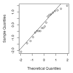
normal probability plot - test scores — **Figure 20:** Normal probability plot test scores

If the normal probability plot points lie reasonably close to the diagonal line, then it is reasonable to assume a normal model for the data. It’s a judgement call, but the normal probability plot points for our test scores (Fig. 20) are quite close to the straight line. Even though the points jump around a bit away from the line, they’re close enough in this case for us to assume a normal model for these test scores.

References

BC Ministry of Health. (2003). Selected vital statistics and health status indicators one hundred thirty-second annual report 2003: Vital Statistics Agency. Retrieved from http://www.vs.gov.bc.ca/stats/annual/2003/index.html

Diez, D. M., Çetinkaya-Rundel, M., Barr, C. D. (2019). OpenIntro Statistics (4^th ed.). OpenIntro. https://www.openintro.org/book/os/

License

Icon for the Creative Commons Attribution-NonCommercial-ShareAlike 4.0 International License

Introduction to Probability and Statistics Copyright © 2023 by Thompson Rivers University is licensed under a Creative Commons Attribution-NonCommercial-ShareAlike 4.0 International License, except where otherwise noted.