Software Lab 4.1

Iain Pardoe

Lesson 4.1: Inference for Proportions

Software Lab 4.1

Inference for Proportions

This software lab is adapted from Inference for Categorical Data (OpenIntro, n.d.-b) CC BY-SA 4.0 at OpenIntro Labs for jamovi.

As you work through the lab, answer the ungraded exercises in the shaded boxes. Check your answers by consulting the Software Lab 4.1 Solutions.

Remember to complete the graded Software Lab Questions for this section in Moodle.

Getting Started: The Data

Every two years, the United States’ Centers for Disease Control and Prevention (CDC) conducts the Youth Risk Behavior Surveillance System (YRBSS) survey, where it takes data from high-schoolers in grades 9 through 12 to analyze health patterns. In this lab, you will work with a selected group of variables from a random sample of observations during one of the years the YRBSS was conducted.

Download the data from yrbss_text [CSV file] (OpenIntro, n.d.-a), and open it in jamovi. The variables are:

gender: Gender of participant; can be male or female.
text_while_driving_30d: During the 30 days preceding the survey, the frequency that participants texted or emailed while driving.
text_ind: Whether the individual texted while driving for six or more days over the preceding 30 days.

We can quickly visualize the distribution of the variable text_while_driving_30d using a frequency table and a bar plot. Do this by selecting Analyses > Exploration > Descriptives and then selecting Frequency tables and Plots > Bar plot. Confirm that the frequency counts are 4,788 for “0 days,” 925 for “1–2 days,” etc.

Confidence Interval for a Single Proportion

First, we’ll focus on the variable text_ind to make inferences about the proportion of US high-schoolers who texted while driving for six or more days over the preceding 30 days. A confidence interval for a single proportion based on a normal model is: $\hat{p} \pm z^* \times \sqrt{\dfrac{\hat{p}(1-\hat{p})}{n}}$ , assuming the following conditions are satisfied:

Independence: The individual responses in the sample are independent of each other.
Random: The sample is random.
Success/Failure Condition: $n\hat{p} \ge 10$ and $n(1-\hat{p}) \ge 10$ .
10% Condition: The sample size $n$ is no more than 10% of the population size.

1. Construct a frequency table for the variable text_ind and use it to check the success/failure condition for the confidence interval. Check your answer by consulting Software Lab 4.1 Solutions.

2. Calculate a 95% confidence interval for the proportion of US high-schoolers who texted while driving for 6 or more days over the preceding 30 days.

Hypothesis Test for a Single Proportion

A journalist claims 15% of US high-schoolers texted while driving for six or more days over the preceding 30 days. We’ll conduct a two-sided hypothesis test for a single proportion to test the journalist’s claim. The hypotheses are H₀: p = 0.15 (15%) versus H_A: p ≠ 0.15. We’ll use a normal model for the sampling distribution of $\hat{p}$ that has a mean of $p_0$ and a standard deviation of $\sqrt{p_0(1-p_0)/n}$ , assuming the following conditions are satisfied:

Independence: The individual responses in the sample are independent of each other.
Random: The sample is random.
Success/Failure Condition: $np_0 \ge 10$ and $n(1-p_0) \ge 10$ .
10% Condition: The sample size $n$ is no more than 10% of the population size.

3. Check the success/failure condition for the hypothesis test.

4. Calculate the test statistic, $Z = \dfrac{\hat{p}-p_0}{\sqrt{\dfrac{p_0(1-p_0)}{n}}}$ .

5. Select Analyses > R > Rj Editor and use the R function pnorm to calculate the p-value. Then, evaluate the hypothesis test based on a significance level $\alpha = 0.05$ and draw a conclusion in the context of the problem.

Inference for a Single Proportion Using the Binomial Model

Section 6.1.4 in the textbook mentions alternate methods for making inferences for a single proportion when the conditions aren’t met, and we can’t use the normal model. One such method is to use the binomial model, as described in Small Sample Hypothesis Testing for a Proportion (Diez et al., 2019) online notes CC BY-SA 3.0.

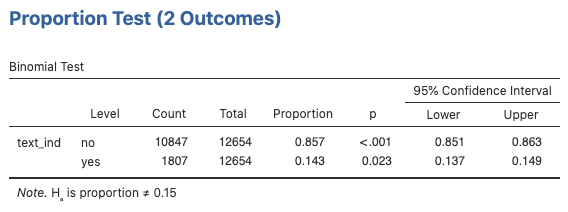
We can use one of jamovi’s built-in tests to conduct a hypothesis test for a proportion using the binomial model as follows. Select Analyses > Frequencies > One Sample Proportion Tests > 2 Outcomes Binomial test and select the test_ind variable. Change Test value to 0.15, and click the Confidence intervals box. The p-value based on the binomial model is in the second row of the resulting binomial test table in the column labeled “p.” The bounds of the corresponding confidence interval are in the last two columns of the table. In this case, the values are the same (to three decimal places) as those based on the normal model (questions 2 and 5 above). They need not match exactly, however, particularly for applications with relatively small sample sizes.

jamovi binomial test — **Figure 1:** Binomial proportion test (two outcomes) in jamovi

Binomial Test
	Level	Count	Total	Proportion	p
text_ind	no	10847	12654	0.857	< .001
	yes	1807	12654	0.143	< .001
Note. Hₐ is proportion ≠ 0.5

Confidence Interval for the Difference Between Two Proportions

Next, we’ll examine whether there is a difference between males and females with respect to the proportion of US high-schoolers who texted while driving for six or more days over the preceding 30 days. A confidence interval for the difference between two proportions based on the central limit theorem is: $\hat{p}_1-\hat{p}_2 \pm z^* \times \sqrt{\dfrac{\hat{p}_1(1-\hat{p}_1)}{n_1}+\dfrac{\hat{p}_2(1-\hat{p}_2)}{n_2}}$ , assuming the following conditions are satisfied:

Independence: The two groups are independent of each other. Within each group, the individual responses are independent of each other.
Random: Each of the two samples is randomly drawn from their respective populations.
Success/Failure Condition: $n_1\hat{p}_1 \ge 10$ , $n_1(1-\hat{p}_1) \ge 10$ , $n_2\hat{p}_2 \ge 10$ , and $n_2(1-\hat{p}_2) \ge 10$ .
10% Condition: Each of the two sample sizes, $n_1$ and $n_2$ , is no more than 10% of their respective population sizes.

6. Construct a frequency table of the variable text_ind split by gender and use it to check the success/failure condition for the confidence interval.

7. Calculate a 95% confidence interval for the difference between the proportion of male US high schoolers who have texted for six or more days while driving over the past 30 days and the proportion of female US high schoolers who have texted for six or more days while driving over the past 30 days.

Hypothesis Test for the Difference Between Two Proportions

Conduct a two-sided hypothesis test to find-out if the population proportions of US high-schoolers who texted while driving for six or more days over the preceding 30 day are equal for males and females. The hypotheses are H₀: p₁ = p₂ versus H_A: p₁ ≠ p₂. We’ll use a normal model for the sampling distribution of $\hat{p}_1-\hat{p}_2$ that has a mean of $p_1-p_2$ and a standard deviation of $\sqrt{\hat{p}(1-\hat{p})\left(\dfrac{1}{n_1}+\dfrac{1}{n_2}\right)}$ , assuming the following conditions are satisfied:

Independence: The two groups are independent of each other. Within each group, the individual responses are independent of each other.
Random: Each of the two samples is randomly drawn from their respective populations.
Success/Failure Condition: $n_1\hat{p} \ge 10$ , $n_1(1-\hat{p}) \ge 10$ , $n_2\hat{p} \ge 10$ , and $n_2(1-\hat{p}) \ge 10$ .
10% Condition: Each of the two sample sizes, $n_1$ and $n_2$ , is no more than 10% of their respective population sizes.

8. Check the success/failure condition for the hypothesis test.

9. Calculate the test statistic, $Z = \dfrac{\hat{p}_1-\hat{p}_2}{\sqrt{\hat{p}(1-\hat{p})\left(\dfrac{1}{n_1}+\dfrac{1}{n_2}\right)}}$ .

10. Select Analyses > R > Rj Editor and use the R function pnorm to calculate the p-value. Then, evaluate the hypothesis test based on a significance level $\alpha = 0.05$ and draw a conclusion in the context of the problem.

We can also use one of jamovi’s built-in tests to conduct a hypothesis test for the difference between two proportions. Select Analyses > Frequencies > Independent Samples > test of association, and select gender for the rows and text_ind for the columns. Click “Statistics” and select z test for difference in 2 proportions under “Tests,” and difference in proportions and confidence intervals under “Comparative Measures.” Confirm the lower and upper bounds of the confidence interval for question 7, the test statistic value from question 9, and the p-value from question 10.

References

Diez, D.M., Çetinkaya-Rundel, M., Barr, C. D. (2019). Small sample hypothesis testing for a proportion [Online supplement]. In, OpenIntro statistics (4^th ed.). http://www.openintro.org/redirect.php?go=stat_sim_prop_ht&referrer=os4_pdf

OpenIntro. (n.d.-a). Data sets [Data sets]. https://openintro.org/data/

OpenIntro. (n.d.-b) CC BY-SA 4.0. Inference for categorical data. OpenIntro Labs for jamovi. https://openintro.shinyapps.io/inf_for_categorical_data_jamovi/

License

Icon for the Creative Commons Attribution-ShareAlike 4.0 International License