Software Lab 4.3

Chi-Square Test of Independence

Is Handedness Independent of Eye Colour?

Consider the example in Supplementary Notes 4.3. Eye colour and handedness were recorded for 114 students. Download the data from eyehand [CSV file] and open it in jamovi. The variable eye records eye colour (brown, blue, green, or other), while the variable hand records handedness (left or right).

Visualize the distribution of the variables eye and hand using a contingency table by selecting Analyses > Exploration > Descriptives. Move eye to the Variables box and hand to the Split by box, and select Frequency tables. Confirm that the observed cell frequencies match those in Supplementary Notes 4.3, i.e., seven for “blue/left,” 26 for “blue/right,” etc.

Since some of the expected cell frequencies are less than five, we have to combine some categories in order to satisfy this condition. Click the data tab and double-click the top of the empty column next to the hand variable to create a new transformed variable. Name it eye2, select eye as the Source variable, and under using transform select Create New Transform. Use the following formula to define the transformation: IF($source=="blue","blue",IF($source=="brown","brown","greenother")). If you’ve done this correctly, you should see a new variable in the spreadsheet called eye2 with values: blue, greenother, blue, brown, etc.

3. Confirm that the value of the test statistic and the p-value in the test output match the values given in Supplementary Notes 4.3.

Are Different Types of Risky Behaviour Independent?

We’ll use data from the United States’ Centers for Disease Control and Prevention Youth Risk Behavior Surveillance System (YRBSS) survey from Software Lab 4.1 to investigate this question. Download the data from yrbss_texthelmet [CSV file] (OpenIntro, n.d.), and open it in jamovi. The variables are:

• text_while_driving_30d: During the 30 days preceding the survey, how frequently the participant texted or emailed while driving.
• helmet_12m: During the 12 months preceding the survey, how frequently the participant wore a helmet while riding a bicycle.

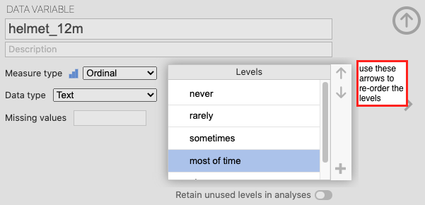
These variables are set as “nominal” by default in jamovi. However, we want to change the measure type to “ordinal” for this lab. Go to the Data tab and double-click the header for helmet_12m. You should see details of the variable; change the Measure type from Nominal to Ordinal. Then use the arrows in the Levels box to re-order the levels into the order: never, rarely, sometimes, most of time, always.

Repeat this process to change the measure type for text_while_driving_30d to nominal and re-order the levels into the order: 0, 1–2, 3–5, 6–9, 10–19, 20–29, 30.

Next, visualize the distribution of the variables text_while_driving_30d and helmet_12m using a contingency table by selecting Analyses > Exploration > Descriptives, moving text_while_driving_30d to the Variables box and helmet_12m to the Split by box, and selecting Frequency tables.

6. Report the value of the test statistic, in the test output in jamovi.

9. Evaluate the hypothesis test based on a significance level and draw a conclusion in the context of the problem.

10. Which combinations of the variables text_while_driving_30d and helmet_12m give rise to the largest standardized difference between observed and expected frequency, ? Hint: To answer this fully, you would need to do this calculation for all 24 combinations, which is pretty tedious. To answer this more intuitively, view the table of observed and expected frequencies in jamovi and look for the most noteworthy differences.