Lesson 4.3: Testing Independence in Two-way Tables
Software Lab 4.3 Solutions
- The expected frequencies for green/left and other/left are 3.83 and 2.67, respectively, so they are not all at least five.
- The expected frequencies are now all at least five.
- The test statistic in the jamovi test output is 0.708, and the p-value is 0.702:
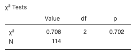
Figure 1: Chi-square test for independence - The observed frequencies are:
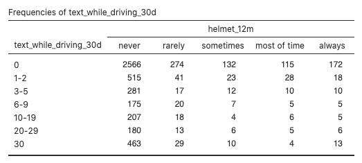
Figure 2: Observed frequencies (never, rarely, sometimes, most of time, always) of the text_while_driving_30d variable - The expected frequencies are all at least five:
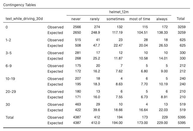
Figure 3: Contingency table shows observed and expected frequencies (never, rarely, sometimes, most of time, always) for text_while_driving_30d  .
.- Degrees of freedom = (7 − 1)(5 − 1) = 6 x 4 = 24, which matches the value in the jamovi output.
- p-value
 .
. - Since p-value
 , there is sufficient evidence to reject the null hypothesis. The data do not support the claim that the variables
 text_while_driving_30dandhelmet_12mare independent. - The following combinations have the largest standardized differences between observed and expected frequency,
 .
.
More than expected: high-schoolers who always wore a helmet and never texted while driving (172 observed, 138.33 expected). Fewer than expected: high-schoolers who never wore a helmet and never texted while driving (2,566 observed, 2,650 expected).
More than expected: high-schoolers who never wore a helmet and texted every day while driving (463 observed, 422 expected). Fewer than expected: high-schoolers who wore a helmet most of the time and texted every day while driving (4 observed, 16.64 expected).
R can do the necessary calculations to find the largest standardized differences between observed and expected frequency,, with the following code (use Analyses > R > Rj Editorto run this code in jamovi):
x <- c(2566,274,132,115,172,515,41,23,28,18,281,17,12,10,10,175,20,7,5,5,207,18,4,6,5,180,13,6,5,6,463,29,10,4,13)

obs <- t(matrix(x, nrow=5))

test <- chisq.test(obs, correct=FALSE)

round(test$residuals, 1)
