Supplementary Notes 5.2

Iain Pardoe

Lesson 5.2: Inference for Difference in Means from Two Independent Groups

Supplementary Notes 5.2

Comparing Means in Independent Groups

Let’s consider media coverage and academic research on the efficacy of weight-loss pills.

Weight-Loss Pills Actually Work, Study Finds

Those given supplement lost weight, while placebo group put on pounds

The Vancouver Sun, Dec. 23, 2006

TORONTO – It almost seems too good to be true.

A study shows that a popular over-the-counter weight-loss supplement can actually help people burn off fat — even during the holiday season when they tend to eat more and exercise less.

For the study, researchers at the University of Guelph and the University of Wisconsin-Madison recruited 40 over-weight but otherwise health volunteers.

Half of them were given a daily supplement of 3.2 grams of conjugated linoleic acid (CLA) for a six-month period that overlapped with the year-end holiday season. The others got inactive placebo pills.

During the course of the study, the CLA group lost a total of 2.2 pounds of fat — especially around the belly.

By contrast, those in the placebo group gained 1.5 pounds during the period from November to December.

The following research (Larsen et al., 2006) was published in The American Journal of Clinical Nutrition.

Conjugated Linoleic Acid Supplementation for 1 y Does Not Prevent Weight or Body Fat Regain (Larsen et al., 2006)

Background: Conjugated linoleic acid (CLA) is marketed as a safe, simple, and effective dietary supplement to promote the loss of body fat and weight. However, most previous studies have been of short duration and inconclusive, and some recent studies have questioned the safety of long-term supplementation with CLA.

Objective: Our aim was to assess the effect of 1-y supplementation with CLA (3.4 g/d) on body weight and body fat regain in moderately obese people.

Design: One hundred twenty-two obese healthy subjects with a body mass index (in kg/m2) > 28 underwent an 8-wk dietary run-in with energy restriction (3300-4200 kJ/d). One hundred one subjects who lost >8% of their initial body weight were subsequently randomly assigned to a 1-y double-blind CLA (3.4 g/d; n = 51) or placebo (olive oil; n = 50) supplementation regime in combination with a modest hypocaloric diet of -1250 kJ/d. The effects of treatment on body composition and safety were assessed with the use of dual-energy X-ray absorptiometry and with blood samples and the incidence of adverse events, respectively.

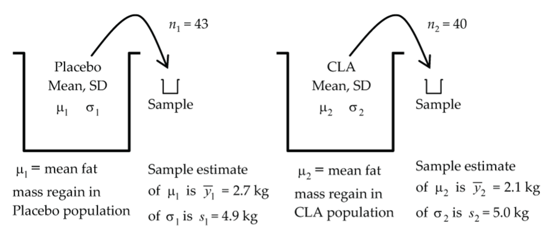
Results: After 1 y, no significant difference in body weight or body fat regain was observed between the treatments. The CLA group (n = 40) regained a mean (+/-SD) 4.0 +/- 5.6 kg body weight and 2.1 +/- 5.0 kg fat mass compared with a regain of 4.0 +/- 5.0 kg body weight and 2.7 +/- 4.9 kg fat mass in the placebo group (n = 43) ….

Conclusion: A 3.4-g daily CLA supplementation for 1 y does not prevent weight or fat mass regain in a healthy obese population.

So, do weight-loss pills really work?

The answer seems to depend on what you mean by “work.” The study reported on in the media article suggests pills do work in helping overweight people lose weight, but the Larsen et al. (2006) study concludes that they are not effective in keeping the weight loss off. Our mission in this lesson is not to resolve whether weight loss pills work; rather, our goal is to develop confidence intervals and tests of hypotheses for comparing the mean response from one group to the mean response from a second group (like mean fat loss/regain CLA vs. placebo).

Our development will parallel that of the difference between two proportions in Supplementary Notes 4.1, only now we’re looking at the difference between two means rather than the difference between two proportions.

Confidence Interval for the Difference Between Two Means

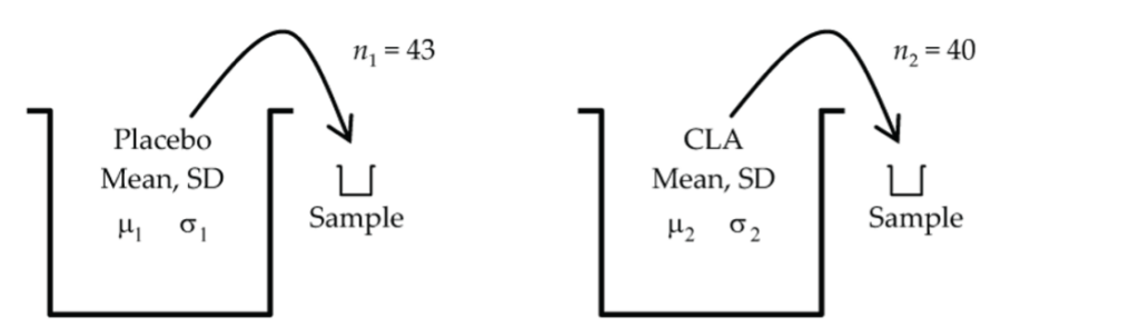
The schematic in Figure 1 illustrates the independent-samples two-mean experimental situation as applied to the fat mass regain variable presented in the Larsen et al. (2006) journal abstract.

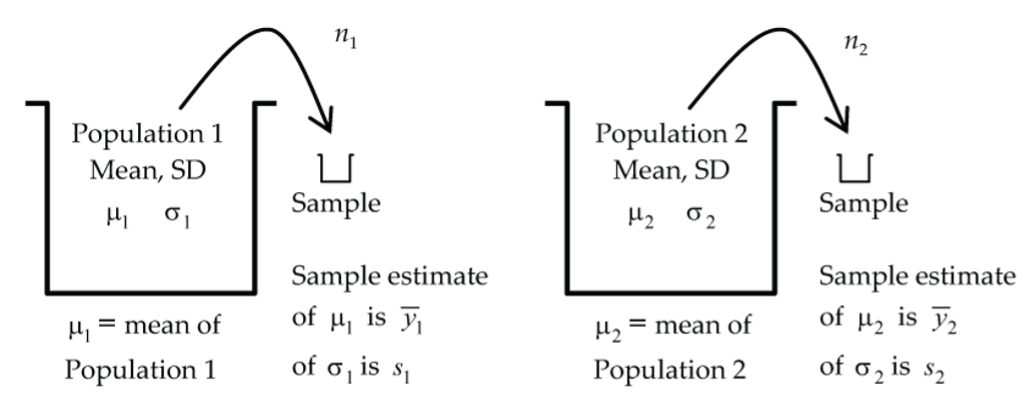
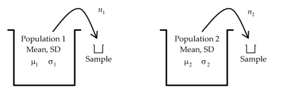
**Figure 1:** Independent samples experiment: Samples are taken from a placebo population and a CLA population.

**Figure 1:** Independent samples experiment: Samples are taken from a placebo population and a CLA population. **new**

Our first goal is to develop a confidence interval for the difference, $\mu_1-\mu_2$ . This CI will have the basic form sample estimate ± margin of error; i.e., $\overline{y}_1-\overline{y}_2$ ± margin of error. This margin of error depends on the sampling distribution of $\overline{y}_1-\overline{y}_2$ .

Under certain conditions (we’ll get to these later), we know that $\overline{y}_1$ has a $N\left( \mu_1, \dfrac{\sigma_1}{\sqrt{n_1}} \right)$ normal model and $\overline{y}_2$ has a $N\left( \mu_2, \dfrac{\sigma_2}{\sqrt{n_2}} \right)$ normal model.

It turns out that the difference $\overline{y}_1-\overline{y}_2$ also has a normal model centred at $\mu_1-\mu_2$ and with standard deviation equal to $\sqrt{\dfrac{\sigma_1^2}{n_1}+\dfrac{\sigma_2^2}{n_2}}$ .

But, the population standard deviations, $\sigma_1$ and $\sigma_2$ are unknown, so we replace them with their corresponding sample estimates, $s_1$ and $s_2$ , and, just like previously, we compensate for the resulting additional uncertainty by using a t-value in place of the normal model z-value.

The confidence interval is therefore $(\overline{y}_1-\overline{y}_2) \pm t^* \times \sqrt{\dfrac{s_1^2}{n_1}+\dfrac{s_2^2}{n_2}}$ .

How many degrees of freedom? There is a complicated formula that appears later in these notes, but it’s usually just a little less than $(n_1-1)+(n_2-1)$ , which is 43 + 40 − 2 = 81 in this example. The complicated df formula later in these notes gives 80.3 df here. Using R, qt(0.975, 80.3) ≈ 1.99.

Sometimes, rather than using degrees of freedom given by the complicated df formula, a conservative approach is taken by using the smaller of $n_1-1$ or $n_2-1$ . In this case, that would mean using df = 39. Using R, qt(0.975, 39) ≈ 2.023. This is conservative because it leads to a slightly wider interval.

Let’s sub-in the numbers for the fat mass regain study to get a 95% CI for the difference in the means for the placebo and CLA supplement:

$(\overline{y}_1-\overline{y}_2) \pm t^* \times \sqrt{\dfrac{s_1^2}{n_1}+\dfrac{s_2^2}{n_2}}$
$(2.7-2.1) \pm 1.99 \times \sqrt{\dfrac{4.9^2}{43}+\dfrac{5.0^2}{40}}$
$0.6 \pm 1.99 \times 1.088$
$0.6 \pm 2.16$
$(-1.56, 2.76)$ kg.

Based on this study, we are 95% confident that the difference in mean fat regains (placebo − CLA) is between –1.56 kg and 2.76 kg. Said another way, the mean fat regain for the placebo population is between 1.56 kg below that of the CLA population and up to 2.76 kg above it. Since this interval contains zero, it can also be interpreted that the two means are not statistically significantly different at the 5% significance level, which is what the abstract correctly concluded.

Sampling Distribution of the Difference Between Two Means

Under what conditions can we use Student’s t-model for comparing two means?

**Figure 2:** Sampling means from two independent groups: Population 1 and Population 2

**Figure 2**: Sampling means from two independent groups: Population 1 and Population 2 **new**

Essentially, we need the same conditions as for the single mean case, but now they must apply to each of our two samples, plus we need one more condition: That the two groups are independent. Here is the complete list of necessary conditions, and by now they should sound familiar!

Conditions

Independence Between Groups: The two groups that we are comparing are independent of each other. This means that there is no linkage or association between the two groups. This would be the case in a completely randomized experiment where the two groups are formed at random, but would not be the case if we used twin pairs, for example, to form the two groups.
Independence Within Groups: Within each group, the individual measurements are independent of each other.
Random: Each of the two samples is randomly drawn from their respective populations.
Nearly Normal Condition: For each of the two samples, the data come from a population that is nearly normal. This condition is important for small data sets, but if each sample is relatively large (say > 30), we don’t have to worry about it too much.
10% Condition: Each of the two sample sizes, n₁ and n₂, is no more than 10% of their respective population sizes

Under these conditions, the sampling distribution of $t = \dfrac{(\overline{y}_1-\overline{y}_2)-(\mu_1-\mu_2)}{\sqrt{\dfrac{s_1^2}{n_1}+\dfrac{s_2^2}{n_2}}}$ can be modeled by Student’s t-model with degrees of freedom given by $df = \dfrac{\left( \dfrac{s_1^2}{n_1}+\dfrac{s_2^2}{n_2} \right)^2}{\dfrac{1}{n_1-1}\left( \dfrac{s_1^2}{n_1} \right)^2 + \dfrac{1}{n_2-1}\left( \dfrac{s_2^2}{n_2} \right)^2}$ .

Example 1: Two-Sample t-Test for the Difference Between Two Means

The data below give the weight losses (in kg) of 15 overweight patients where eight were randomly assigned to the treatment group and seven to the placebo group.

Treatment: 4.1, 8.8, 7.4, 6.7, 5.5, 4.8, 6.4, 3.2
Placebo: 4.8, 1.8, 2.8, 3.1, 2.5, 0.5, 3.6

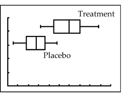
Boxplots - weight loss — **Figure 3:** Boxplots for weight loss treatment and placebo groups

Is there sufficient evidence to conclude that the mean weight loss for the treatment group is higher than that for the placebo group?

Hypotheses

H₀: µ_treatment = µ_placebo (or equivalently µ_treatment – µ_placebo = 0); i.e., no difference in the population mean weight losses
H_A: µ_treatment ≠ µ_placebo (or equivalently µ_treatment – µ_placebo ≠ 0)

Conditions

Independence Between Groups: Yes, since the two groups were created randomly.
Independence Within Groups: No way to judge, but reasonable to assume.
Random: Not stated how the 15 overweight patients were selected. This could be an issue.
Nearly Normal Condition: We could do a normal probability plot for each sample, but the two boxplots (Fig. 3) show sample distributions that are reasonably symmetric and concentrated in the middle, so it is reasonable to assume each sample comes from a normal model.
10% Condition: Each of the two sample sizes is well below 10% of all overweight patients.

Mechanics

Since the mechanics are now getting complicated, let’s turn the computational details over to jamovi.

Download the data weightloss [CSV file], and open it in jamovi.
Click the data tab and double-click the header for the group variable. Re-order the levels so treatment is first and control is second.
Select Analyses > T-Tests > Independent Sample T-Test.
Move loss to the Dependent Variables box and group to the Grouping Variable box.
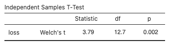
Select Welch's under Tests (and unselect Student's if it is selected, since this uses the pooled standard deviation that assumes equal population standard deviations in both groups).
The test statistic (3.79), degrees of freedom (12.7), and p-value (0.002) are given in the Independent Sample T-test output.

Independent sample t-test - weight loss — **Figure 4:** Independent sample t-test for weight loss

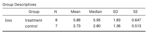
Select Descriptives to see the sample statistics, e.g., the group means (5.86 for treatment and 2.73 for control).

Sample statistics - weight loss — **Figure 5:** Sample statistics for weight loss data

Conclusion

If the two population mean losses were equal (H₀ true), there is only a two in 1,000 chance that we’d get a treatment sample mean that is 3.13 kg (5.86 − 2.73) or more different than the placebo mean. Too unusual (less than significance level $\alpha=0.05$ ), so reject H₀. Since the sample mean for treatment is higher than for control, conclude that the mean weight loss for the treatment group is higher than the mean weight loss for the placebo group.

Alternatively, reject H₀ in favour of H_A if the test statistic is in the rejection region (either less than the negative critical value or greater than the positive critical value). Do not reject H₀ if the test statistic is not in the rejection region (i.e., it is between the negative and positive critical values). The critical value in the weight loss example is 2.1656, the 97.5^th percentile of the t-distribution with 12.7 degrees of freedom. Since the test statistic, $t=3.79$ is greater than 2.1656, it is in the rejection region, so we reject H₀ in favour of H_A.

Example 2: Two-Sample t-Interval for the Difference Between Two Means

We used the two-sample t-test to conclude that the mean weight loss for the treatment group is statistically significantly higher than the mean weight loss for the placebo group. But, how much higher is it?

Let’s answer this by calculating a 95% confidence interval for the difference between these means. Since we’ve already checked the conditions, let’s move directly to the calculations. Again, jamovi makes the calculations easy.

Select Mean difference and Confidence interval in the Independent Samples T-Test dialog.

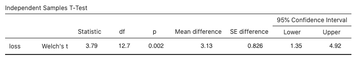
Independent Samples Confidence Interval - weight loss — **Figure 6:** Independent samples confidence interval of weight loss data

We are 95% confident that the mean weight loss for the treatment group is between 1.35 kg to 4.92 kg greater than the mean weight loss for the placebo group.

Hand calculation, anyone?

Just to prove that we can do it, let’s do the “by hand” calculation of the above CI (using the sample statistics).

$df= \dfrac{\left( \dfrac{s_1^2}{n_1}+\dfrac{s_2^2}{n_2} \right)^2}{\dfrac{1}{n_1-1}\left( \dfrac{s_1^2}{n_1} \right)^2 + \dfrac{1}{n_2-1}\left( \dfrac{s_2^2}{n_2} \right)^2} = \dfrac{\left( \dfrac{1.83^2}{8}+\dfrac{1.36^2}{7} \right)^2}{\dfrac{1}{7}\left( \dfrac{1.83^2}{8} \right)^2 + \dfrac{1}{6}\left( \dfrac{1.36^2}{7} \right)^2} = 12.7$ .
Using R, qt(0.975, 12.7) ≈ 2.166.
$(\overline{y}_1-\overline{y}_2) \pm t^* \times \sqrt{\dfrac{s_1^2}{n_1}+\dfrac{s_2^2}{n_2}} = (5.86-2.73) \pm 2.166 \times \sqrt{\dfrac{1.83^2}{8}+\dfrac{1.36^2}{7}}$ $= 3.13 \pm 2.166(0.826) = 3.13 \pm 1.79 = (1.34, 4.92)$ kg.

The “by hand” CI differs slightly from that given by the calculator due to round-off error in the CI and df calculations.

Example 3: Two-Sample t-Test for the Difference Between Two Means

Read this excerpt from the abstract of a research article (Dunstan et al., 2008).

Cognitive Assessment of Children at Age 2½ Years After Maternal Fish Oil Supplementation in Pregnancy: A Randomised Controlled Trial (Dunstan et al., 2008)

Objective: To assess the effects of antenatal omega 3 long chain polyunsaturated fatty acid on cognitive development in a cohort of children whose mothers received high dose fish oil in pregnancy.

Design: A double-blind randomised placebo-controlled trial.

Setting: Perth, Western Australia.

Patients: Pregnant women (n = 98) received the supplementation from 20 weeks gestation until delivery. Their infants (n = 72) were assessed at 2½ years of age.

Interventions: Fish oil (2.2g docosahexaenoic acid (DHA) plus 1.1g eicosapentaenoic acid (EPA)/day) or olive oil from 20 weeks gestation until delivery.

Main Outcome Measures: Effects on infant growth and developmental quotients (Griffiths Mental Development Scales), receptive language (Peabody Picture Vocabulary Test) and behaviour (Child Behaviour Checklist).

Results: Children in the fish oil-supplemented group (n = 33) attained a significantly higher score for eye and hand coordination (mean score 114, SD 10.2) than those in the placebo group (n = 39, mean score 108, SD 11.3) (p = 0.021) ….

Conclusion: Maternal fish oil supplementation during pregnancy is safe for the fetus and infant, and may have potentially beneficial effects on the child’s eye and hand coordination. Further studies are needed to determine the significance of this finding.

Note: Reproduced from Archives of Disease in Childhood – Fetal and Neonatal Edition, Dunstan, J. A., Simmer, K., Dixon, G., & Prescott, S.L., volume 93, pF45-F50, ©2008 with permission from BMJ Publishing Group Ltd.

This abstract presents very clearly the “Why, How, Where, Who, What” aspects of a completely randomized experiment comparing two means. Let’s use the two-sample t-test to confirm the p-value calculation quoted in the results section.

Hypotheses

H₀: µ_fishoil = µ_placebo (or equivalently µ_fishoil – µ_placebo = 0); i.e., no difference in the population mean eye-hand coordination score
H_A: µ_fishoil ≠ µ_placebo (or equivalently µ_fishoil – µ_placebo ≠ 0)

Conditions

Independence Between Groups: Yes, since the two groups were created randomly.
Independence Within Groups: No way to judge, but reasonable to assume.
Random: Not stated how the pregnant women were selected. This could be an issue.
Nearly Normal Condition: No way to judge with only the summary information on the sample means and SDs. Sample sizes (33, 39) are reasonably large, so unless the data were badly skewed or outliers present, we need not worry about the nearly normal condition.
10% Condition: Each of the two sample sizes is well below 10% of all pregnant women.

Hand Calculation

$t = \dfrac{(\overline{y}_1-\overline{y}_2)-(\mu_1-\mu_2)}{\sqrt{\dfrac{s_1^2}{n_1}+\dfrac{s_2^2}{n_2}}} = \dfrac{(114-108)}{\sqrt{\dfrac{10.2^2}{33}+\dfrac{11.3^2}{39}}} = 2.37$ .
$df= \dfrac{\left( \dfrac{s_1^2}{n_1}+\dfrac{s_2^2}{n_2} \right)^2}{\dfrac{1}{n_1-1}\left( \dfrac{s_1^2}{n_1} \right)^2 + \dfrac{1}{n_2-1}\left( \dfrac{s_2^2}{n_2} \right)^2} = \dfrac{\left( \dfrac{10.2^2}{33}+\dfrac{11.3^2}{39} \right)^2}{\dfrac{1}{32}\left( \dfrac{10.2^2}{33} \right)^2 + \dfrac{1}{38}\left( \dfrac{11.3^2}{39} \right)^2} = 69.7$ .
P-value, 2 * (1 - pt(2.37, df=69.7)) ≈ 0.021.

Conclusion

The p-value of 0.021 quoted in the abstract is confirmed, and the conclusion that the fish-oil group attained a (statistically) significantly higher mean eye-hand score follows.

Alternatively, reject H₀ in favour of H_A if the test statistic is in the rejection region (either less than the negative critical value or greater than the positive critical value). Do not reject H₀ if the test statistic is not in the rejection region (i.e., it is between the negative and positive critical values). The critical value in the fish-oil example is 1.9946, the 97.5^th percentile of the t distribution with 69.7 degrees of freedom. Since the test statistic, $t=2.37$ is greater than 1.9946, it is in the rejection region, so we reject H₀ in favour of H_A.

References

Dunstan, J. A., Simmer, K., Dixon, G., & Prescott, S.L. (2008). Cognitive assessment of children at age 2(1/2) years after maternal fish oil supplementation in pregnancy: a randomised controlled trial. Archives of Disease in Childhood – Fetal and Neonatal Edition, 93(1), F45-F50. https://doi.org/10.1136/adc.2006.099085

Larsen, T. M., Toubro, S., Gudmundsen, O., & Astrup, A. (2006). Conjugated linoleic acid supplementation for 1 y does not prevent weight or body fat. American Journal of Clinical Nutrition, 83(3), 606–612. DOI: 10.1093/ajcn.83.3.606

Weight-loss pills actually work, study finds: Those given supplement lost weight, while placebo group put on pounds. (2006, December 23). The Vancouver Sun. https://advance.lexis.com/api/document?collection=news&id=urn:contentItem:4MMW-JF30-TWD4-01R9-00000-00&context=1516831

License

Icon for the Creative Commons Attribution-NonCommercial-ShareAlike 4.0 International License

Introduction to Probability and Statistics Copyright © 2023 by Thompson Rivers University is licensed under a Creative Commons Attribution-NonCommercial-ShareAlike 4.0 International License, except where otherwise noted.

Comparing Means in Independent Groups

Weight-Loss Pills Actually Work, Study Finds

Conjugated Linoleic Acid Supplementation for 1 y Does Not Prevent Weight or Body Fat Regain (Larsen et al., 2006)

Confidence Interval for the Difference Between Two Means

Sampling Distribution of the Difference Between Two Means

Conditions

Example 1: Two-Sample t-Test for the Difference Between Two Means

Hypotheses

Conditions

Mechanics

Conclusion

Example 2: Two-Sample t-Interval for the Difference Between Two Means

Example 3: Two-Sample t-Test for the Difference Between Two Means

Cognitive Assessment of Children at Age 2½ Years After Maternal Fish Oil Supplementation in Pregnancy: A Randomised Controlled Trial (Dunstan et al., 2008)

Hypotheses

Conditions

Hand Calculation

Conclusion

References

License

Share This Book