Supplementary Notes 5.3

Iain Pardoe

Lesson 5.3: Inference for Multiple Means Using ANOVA

Supplementary Notes 5.3

Baseball Batting Performance

Consider the example in Section 7.5.2 of the textbook that asks the question: Is batting performance related to player position in Major League Baseball (MLB)?

The data in bat18 [CSV file] includes batting records of 429 MLB players from the 2018 season who had at least 100 “at bats.” The variables in this study are:

OBP: on-base percentage, which is roughly equal to the fraction of times a player gets on base or hits a home run.
position: the player’s primary field position (OF for outfield, IF for infield, C for catcher).

OBP is our response variable, y, in this study, and position is our explanatory group variable. Figure 1 has boxplots of OBP for each position:

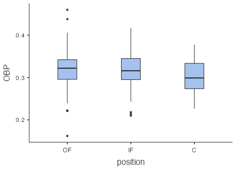
boxplots - mlb batting example — **Figure 1**: Boxplots for MLB on-base percentage (OBP) by player position (outfield is OF; infield is IF; and catcher is C).

Figure 2 presents summary statistics of OBP for each position:

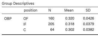
summary statistics - mlb batting example — **Figure 2**: Group descriptives for MLB batting results by player position (outfield is OF; infield is IF; and catcher is C).

Based on the boxplot distributions (Fig. 1) and the summary statistics (Fig. 2), it looks like batting performance (as measured by OBP) is better for outfielders, then infielders, then catchers. We might wonder then if, based on this sample of players, we can conclude that the population mean OBP is higher for outfielders, then infielders, then catchers? However, there’s a fair bit of variability in y (OBP) within each group (position), so statistically we need to ask whether there is sufficient variation in the sample group means relative to the sample variation of y within each group to conclude there is a difference in the population group means.

We answer this question using a technique called Analysis of Variance (ANOVA), which uses a new family of models called F models.

F Models

F models, like the chi-square models introduced in Supplementary Notes 4.2, only take positive values and are skewed to the right. They use a probability distribution called the F-distribution that has two degrees of freedom numbers:

df₁ is called the numerator degrees of freedom.
df₂ is called the denominator degrees of freedom.

Analysis of Variance (ANOVA)

Here’s how to conduct Fisher’s ANOVA F-test to compare population means in k groups.

Hypotheses

H₀: The mean response is the same across all k groups, i.e., $\mu_1=\mu_2=\dots=\mu_k$ .
H_A: At least two means are different.

Conditions

Independence: The observations are independent within and between groups.
Nearly Normal Condition: The observations within each group are nearly normal. If the observations are highly non-normal, then use a Kruskal-Wallis test instead. (Details are beyond the scope of this course.)
Variability: The variability within each group is approximately the same. If the within-group variability is too different, then use Welch’s ANOVA instead. (Details are beyond the scope of this course.)

Mechanics

Use statistical software to obtain the test statistic, .
- $MSG$ is the mean square between groups and measures variability between the group means ( $\overline{y}_1, \overline{y}_2, \dots, \overline{y}_k$ ).
- $MSE$ is the mean square error and measures variability in y within the groups.
Use statistical software to obtain the p-value using the fact that under the null hypothesis, $F$ has an F-distribution with $k-1$ numerator degrees of freedom (df₁) and $n-k$ denominator degrees of freedom (df₂).

Decision Rule and Conclusion

If the p-value is less than the significance level $\alpha$ , then reject H₀ in favour of H_A and conclude that there is sufficient evidence that at least two population means are different.
If the p-value is greater than the significance level $\alpha$ , then fail to reject H₀ in favour of H_A and conclude that there is insufficient evidence that at least two population means are different.

Baseball Example

Hypotheses

H₀: $\mu_1=\mu_2=\mu_3$ .
H_A: At least two means are different.

Conditions

Independence: No obvious reason to doubt independence within and between groups.
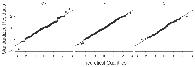
Nearly Normal Condition: The observations within each group appear to be nearly normal based on the points lying reasonably close to the lines in the following normal probability plots, with no extreme outliers.

normal probability plots - mlb batting example — **Figure 3**: Normal probability plots for MLB player batting: outfield players (OF); infield players (IF); and catchers (C)

Variability: The variability within each group is approximately the same based on the sample statistics reported above.

Mechanics

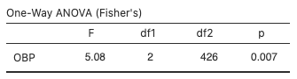
From the jamovi software output (Fig. 4), $F = 5.08$ .
The p-value based on the F-distribution with $2$ numerator degrees of freedom (df₁) and $426$ denominator degrees of freedom (df₂) is 0.007.

anova - mlb batting example — **Figure 4**: One-way ANOVA for MLB player batting

Decision Rule and Conclusion

The p-value 0.007 is less than the significance level $\alpha=0.05$ , so reject H₀ in favour of H_A and we conclude that there is sufficient evidence that at least two population means are different.

Alternatively, reject H₀ in favour of H_A if the test statistic is in the rejection region (greater than the critical value). Do not reject H₀ if the test statistic is not in the rejection region (less than the critical value). The critical value in the baseball example is 3.0169, the 95^th percentile of the chi-square distribution with two numerator degrees of freedom and 426 denominator degrees of freedom. Since the test statistic, F = 5.08 is greater than 3.0169, it is in the rejection region, so we reject H₀ in favour of H_A.

Multiple Comparisons

Having found evidence that at least two population means are different, we might be tempted at this point to use the two-sample t-tests from Lesson 5.2 to determine which means are different from each other. However, that would require multiple tests, each having a chance of leading to an incorrect decision (a Type 1 error), which leads to an excessive risk of concluding that two means are different when they’re really the same. For example, in the baseball example, if we were to do three t-tests each using $\alpha=0.05$ , then the overall probability of concluding that two means are different when they’re really the same is $1-(1-0.05)^3=0.143$ , which is considered unacceptably high.

To mitigate this problem of multiple comparisons, we can try a few different post-hoc approaches, two of which are:

Bonferroni correction for $\alpha$ : Simply divide $\alpha$ by the number of groups (k) and conduct the two-sample t-tests using $\alpha/k$ and the pooled standard deviation based on all k groups. This approach is easy to apply, but it is not the most effective.
Tukey’s range test (or Tukey’s HSD): The specifics of how this works lie beyond the scope of this course. All we need to know is that we can use statistical software to find adjusted p-values for all the pairwise comparisons.

Baseball Example

Bonferroni correction for $\alpha$ : Conduct the two-sample t-tests using $\alpha/k=0.05/3=0.0167$ .

Compare OF to IF: t-statistic = 0.342, p-value = 0.7325 > 0.0167. Conclude not different.
Compare OF to C: t-statistic = 3.04, p-value = 0.0025 < 0.0167. Conclude different.
Compare IF to C: t-statistic = 2.89, p-value = 0.0040 < 0.0167. Conclude different.

Overall conclusion: The mean OBP for outfielders and infielders do not differ statistically, but both differ from the mean OBP for catchers.

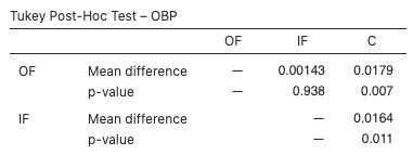
Tukey’s range test (Tukey’s HSD):

Compare OF to IF: mean difference = 0.00143, adjusted p-value = 0.938 > 0.05. Conclude not different.
Compare OF to C: mean difference = 0.0179, adjusted p-value = 0.007 < 0.05. Conclude different.
Compare IF to C: mean difference = 0.0164, adjusted p-value = 0.011 < 0.05. Conclude different.

Overall conclusion: The mean OBP for outfielders and infielders do not differ statistically, but both differ from the mean OBP for catchers.

tukey post-hoc tests: mlb batting example — **Figure 5**: Tukey’s post-hoc test for MLB player batting: outfield players (OF); infield players (IF); and catchers (C)

License

Icon for the Creative Commons Attribution-NonCommercial-ShareAlike 4.0 International License

Introduction to Probability and Statistics Copyright © 2023 by Thompson Rivers University is licensed under a Creative Commons Attribution-NonCommercial-ShareAlike 4.0 International License, except where otherwise noted.

Baseball Batting Performance

F Models

Analysis of Variance (ANOVA)

Hypotheses

Conditions

Mechanics

Decision Rule and Conclusion

Baseball Example

Hypotheses

Conditions

Mechanics

Decision Rule and Conclusion

Multiple Comparisons

Baseball Example

License

Share This Book