Lesson 6.3: Multiple Linear Regression
Supplementary Notes 6.3
Multiple Linear Regression Model
To illustrate the multiple linear regression model, we’ll revisit the Human Freedom Index data from Software Lab 6.2. We’ll use the following variables:
pf_score: Personal Freedom (score): (0) worst – (10) best.pf_media_control: Political pressures and controls on media content: (0) low – (10) high.pf_security_safety: Security and safety: (0) worst – (10) best.pf_women_restrict: Measurement of restrictions on the freedom of women to move outside the home: “none” indicates no restrictions of women’s movement outside the home, “some” indicates (some) women can leave home sometimes with some restrictions, and “severe” indicates women can never leave home without restrictions (i.e., they need a male companion, etc.).
After opening the hfi2016 [CSV file] (OpenIntro, n.d.) data in jamovi, we select Analyses > Regression > Linear Regression, move pf_score to the “Dependent Variable” box, move pf_media_control and pf_security_safety to the “Covariates” box, and move pf_women_restrict to the “Factors” box:
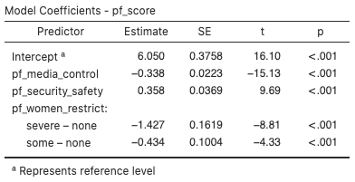
We use the coefficients in the “Estimate” column to write the estimated multiple linear regression equation:

 .
.
Categorical Predictors
The predictor pf_women_restrict is a categorical variable with three categories. We include categorical predictors in a multiple linear regression model by using binary indicator variables that take the value “1” for one category and “0” for the other categories. The number of indicator variables we need is one fewer than the number of categories. Since we have three categories for pf_women_restrict, we need two indicator variables:
pf_women_restrictsevere: 1 if women can never leave home without restrictions, 0 otherwisepf_women_restrictsome: 1 if women can leave home sometimes with some restrictions, 0 otherwise
The category that is left out (no restrictions of women’s movement outside the home) is known as the reference category, and countries in this category have the value “0” for both pf_women_restrictsevere and pf_women_restrictsome.
We plug in 0s and 1s to the estimated regression equation and simplify to derive estimated regression equations for each category of pf_women_restrict:
- Severe:


- Some:


- None:


Interpreting Estimated Coefficients
We interpret an estimated coefficient for a numerical predictor in a multiple linear regression model as the expected change in the response variable for a one-unit increase in the predictor, holding all other predictors fixed. In this case:
- We expect
pf_scoreto decrease by 0.338 for each additional one-unit inpf_media_control, holding all other predictors fixed. - We expect
pf_scoreto increase by 0.358 for each additional one-unit inpf_security_safety, holding all other predictors fixed.
We interpret an estimated coefficient for an indicator variable in a multiple linear regression model as the expected difference in the response variable between the indicated category and the reference category, holding all other predictors fixed. In this case:
- We expect
pf_scoreto be 1.427 lower forpf_women_restrict=severecompared topf_women_restrict=none, holding all other predictors fixed. - We expect
pf_scoreto be 0.434 lower forpf_women_restrict=somecompared topf_women_restrict=none, holding all other predictors fixed.
The estimated intercept represents the expected response variable when all the predictor variables are 0. For this interpretation to be valid, the concept of “all the predictor variables being 0” has to be meaningful and there has to be some data with all the predictor variables at or close to 0. This rarely happens in practice and is not the case in this example.
Explained Variation
The coefficient of variation or R2 measures the percentage of the variation in the response variable (y) that has been accounted for by the linear model.
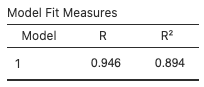
In this case, 89.4% of the variation in personal freedom scores has been accounted for by this multiple linear regression model.
Assumption Checks
In the linear regression analysis, open the “Assumption Checks” sub-menu and check “Q–Q plot of residuals” and “Residual plots.”
- Linearity: There is a slight nonlinear pattern in the “Residuals vs Fitted” plot (Fig. 3), which indicates it may not be reasonable to assume linearity. The next step might be to consider a more complex model with additional predictor variables. (We’ll save that for another course!)
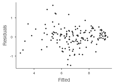
Figure 3: Scatterplot of residuals vs. fitted for Human Freedom Index data - Nearly normal residuals: The majority of the points (Fig. 4) lie close to the diagonal line in the normal probability plot with no extreme outliers, which indicates that the nearly normal residuals condition is not violated.
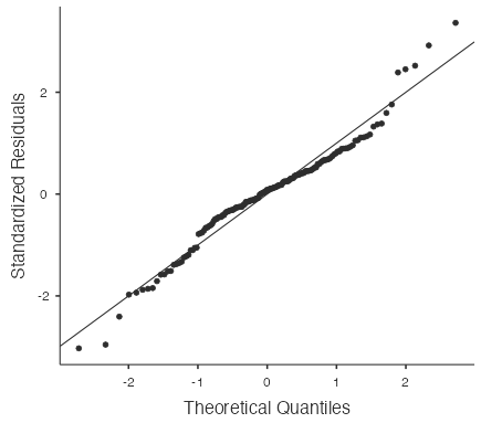
Figure 4: Normal probability plot for Human Freedom Index data - Constant variability: The variability of the residuals in the “Residuals vs Fitted” plot (Fig. 3) appear reasonably constant across the plot, which indicates that the constant variability condition is not violated.
References
OpenIntro. (n.d.). Data sets [Data sets]. https://openintro.org/data/
