Software Lab 2.2

Conditional Probability

This software lab is adapted from the Probability (OpenIntro, n.d.-b) CC BY-SA 4.0 lab at OpenIntro Labs for jamovi.

The Hot Hand

Basketball players who make several baskets in succession are described as having a hot hand. Fans and players have long believed in the hot hand phenomenon, which refutes the assumption that each shot is independent of the next. However, a paper titled The Hot Hand in Basketball: On the Misperception of Random Sequences (Gilovich et al., 1985) collected evidence that contradicted this belief and showed that successive shots are independent events. This paper started a great controversy that continues to this day, as you can see by Googling “hot hand basketball.”

We do not expect to resolve this controversy today. However, in this lab we’ll apply one approach to answering questions like this. The goals for this lab are to: (1) think about the effects of independent and dependent events; (2) learn how to simulate shooting streaks in jamovi; and (3) to compare a simulation to actual data in order to determine if the hot hand phenomenon appears to be real.

Data

Download the kobe_basket [CSV file] (OpenIntro, n.d.-a) data file and load it into jamovi. Our investigation will focus on the performance of one player: Kobe Bryant. He was a star player on the Los Angeles Lakers basketball team. His performance against the Orlando Magic in the 2009 NBA Finals earned him the Most Valuable Player (MVP) title, and many spectators commented on how he appeared to show a hot hand.

This data frame contains 133 observations and 6 variables, where every row records a shot taken by Kobe Bryant. The shot variable in this dataset indicates whether the shot was a hit (H) or a miss (M).

Just looking at the string of hits and misses, it can be difficult to gauge whether or not it seems like Kobe was shooting with a hot hand. One way we can approach this is by considering the belief that hot hand shooters tend to go on shooting streaks. For this lab, we define the length of a shooting streak to be the number of consecutive baskets made until a miss occurs.

For example, in Game 1 Kobe had the following sequence of hits and misses from his nine shot attempts in the first quarter:

H M | M | H H M | M | M | M

You can verify this by viewing the first 9 rows of the data in the data viewer.

Within the nine shot attempts, there are six streaks, which are separated by a “|” above. Their lengths are one, zero, two, zero, zero, zero (in order of occurrence).

Counting streak lengths manually for all 133 shots would get tedious, so we’ll use some code written in the language R, which jamovi is built on, to calculate the lengths of streaks for us.

R Code

You won’t be editing R code directly, but you’ll need to add a module to be able to copy the code into jamovi and then run it. Click the plus button at the top right part of the screen, select jamovi library, then click INSTALL for the Rj - Editor to run R code inside jamovi module. If this module is already installed, it will say INSTALLED and you’re good to go. Click the up arrow to close this menu, then click the new R tab and select Rj Editor. Delete any code that is already there and then copy/paste the code below into the box:

Then click the green play button. You won’t see anything happen, but the computer now knows how to calculate streak lengths. Don’t worry about the specific code syntax here. All you need to know is that this code defines a function in jamovi to calculate streak lengths for any set of data representing a series of Hs and non-Hs. To calculate the actual streak lengths for the kobe_basket data, copy/paste the following text into the same box below what you already typed, and click the play button.

If you’ve done this correctly, you will see a list of all the streak lengths from the data set:

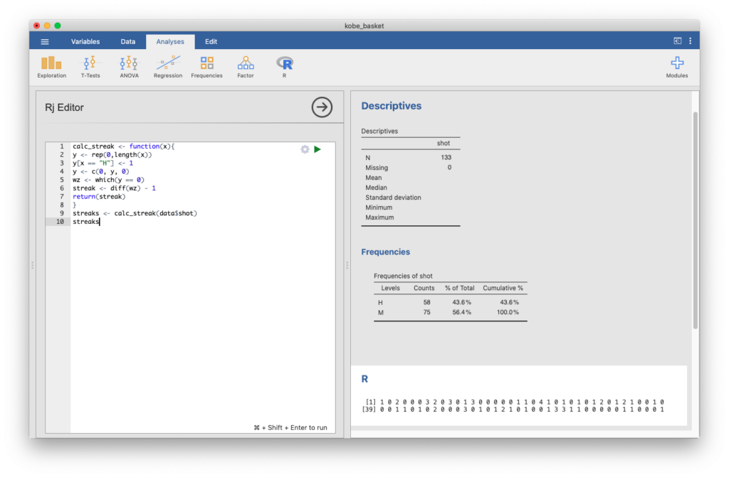
Note that you’ll likely see a number in brackets show up (like [39]). This isn’t an actual streak length, it’s just indicating the 39^th value in the list so you can keep track.

You can find some summary information on the streak lengths and view a histogram using the code:

Add this into the box and run it as well.

Compared to What?

We’ve shown that Kobe had some long shooting streaks, but are they long enough to support the belief that he had a hot hand? What can we compare them to?

To answer these questions, let’s return to the idea of independence. Two processes are independent if the outcome of one process doesn’t effect the outcome of the second. If each shot that a player takes is an independent process, having made or missed your first shot will not affect the probability that you will make or miss your second shot.

A shooter with a hot hand will have shots that are not independent of one another. Specifically, if the shooter makes his first shot, the hot hand model says he will have a higher probability of making his second shot. Let’s suppose for a moment that the hot hand model is valid for Kobe. During his career, the percentage of time Kobe makes a basket (i.e. his shooting percentage) is about 45%. So, for his first shot,

P(shot 1 = H) = 0.45.

If he makes the first shot and has a hot hand (not independent shots), then the conditional probability that he makes his second shot would go up to, let’s say, 60%:

P(shot 2 = H | shot 1 = H) = 0.60.

(Remember, the symbol “|” means “given.”) As a result of these increased probabilities, you’d expect Kobe to have longer streaks. Compare this to the skeptical perspective where Kobe does not have a hot hand, where each shot is independent of the next. If he hit his first shot, the probability that he makes the second is still 0.45:

P(shot 2 = H | shot 1 = H) = 0.45.

In other words, making the first shot did nothing to effect the probability that he’d make his second shot. If Kobe’s shots are independent, then he’d have the same probability of hitting every shot regardless of his past shots: 45%.

Now that we’ve phrased the situation in terms of independent shots, let’s return to the question: how do we tell if Kobe’s shooting streaks are long enough to indicate that he has a hot hand? We can compare his streak lengths to someone without a hot hand, i.e., an independent shooter.

Simulations in jamovi

While we don’t have any data from a shooter we know to have independent shots, that sort of data is very easy to simulate in jamovi. In a simulation, you set the ground rules of a random process and then the computer uses random numbers to generate an outcome that adheres to those rules.

As a simple example, you can simulate flipping a fair coin. You’re going to flip your simulated coin 133 times (because that’s the size of the data set) and see what the results look like.

Create a new variable called by clicking the Data tab, double-clicking the top of the first empty column where the variable name would be, and selecting NEW COMPUTED VARIABLE. Name the variable sim_coin and as the formula for the variable, enter IF(UNIF()<0.5,"H","T").

Before proceeding, let’s unpack this formula: UNIF() picks a random number between 0 and 1. The jamovi software then tests whether the number is less than 0.5. If it’s less, it picks an “H,” otherwise it picks a “T.” It then repeats this process for every row in the data set. This means you’ll see a column of random H’s and T’s, representing the heads and tails of 133 flips of a simulated fair coin.

Each entry in sim_coin can be thought of as a hat with two slips of paper in it: One slip says heads (H) and the other says tails (T). Each entry draws one slip from the hat and tells us if it was a head or a tail. Just like when flipping a coin, sometimes you’ll get a heads, sometimes you’ll get a tails, but in the long run, you’d expect to get roughly equal numbers of each.

We used the default probability that when we “flip” a coin and it lands heads is 0.5. Say we’re trying to simulate an unfair coin that we know only lands heads 20% of the time. We can adjust this by changing when the random number gets assigned an “H” or a “T” in our IF statement. Create another new variable named sim_unfair_coin and assigned it with the function IF(UNIF()<0.2,"H","T"). This will come up heads 20% of the time and tails 80% of the time, on average. Create a table of counts for the results of this simulation. Another way of thinking about this is to think of the outcome space as a bag of 10 chips, where 2 chips are labeled “head” and 8 chips “tail.” Therefore at each draw, the probability of drawing a chip that says “head” is 20%, and “tail” is 80%.

In a sense, we’ve shrunken the size of the slip of paper that says “heads,” making it less likely to be drawn, and we’ve increased the size of the slip of paper saying “tails,” making it more likely to be drawn. When you simulated the fair coin, both slips of paper were the same size.

Simulating the Independent Shooter

Simulating a basketball player who has independent shots uses the same mechanism that you used to simulate a coin flip.

To make a valid comparison between Kobe and your simulated independent shooter, you need to align their shooting percentages.

Now, return to the R window (in the Analyses tab). To calculate and summarize the streak lengths for our new variable, use the code:

You may need to first re-run the previous code used to set-up the function for calculating streak lengths.

More Practice

Comparing Kobe Bryant to the Independent Shooter

You now have the data necessary to compare Kobe to our independent shooter. Both data sets represent the results of 133 shot attempts, each with the same shooting percentage of 45%. We know that our simulated data is from a shooter that has independent shots. That is, we know the simulated shooter does not have a hot hand.