Supplementary Notes 1.2

Sample Surveys, Observational Studies, and Experiments

Consider the following newspaper article (Herring, 2021) published by Calgary Herald.

Imagine that you were charged with the task of conducting a survey to investigate the extent and nature of student cheating at Canadian universities. A rather overwhelming task, isn’t it!

• • How do you actually go about selecting the students to be interviewed?
  • How many students should be interviewed?
  • What questions should be asked?

Population vs. Sample

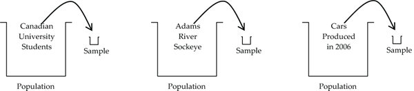
The basic goal of a sample survey is to “learn something” about a large population. It could be a “people population” (e.g., Canadian university students), a “fish population” (e.g., the total Adams River sockeye salmon run), or a “car population” (e.g., all new cars produced in a given year). We collect a sample from the population that typically is very much smaller in size compared to the population. Based on the sample information we make estimates and inferences for the population.

What does it mean by saying the goal is to “learn something”?

Let’s get more specific. Usually, we are trying to learn something about some parameter of the population, and we use a corresponding sample statistic to estimate the population parameter.

The following list shows the most common population parameters of interest in a study along with their corresponding sample statistic estimate. Also notice that we use different symbols to distinguish population parameters from their corresponding sample statistic estimates.

Possible Population Parameters of Interest	Corresponding Sample Statistics
population mean, (“mu”)	sample mean, (“y-bar”)
population standard deviation, (“sigma”)	sample standard deviation, s
population proportion, p	sample proportion,  (“p-hat”)

For example, the Calgary Herald story (Herring, 2021) reported global, self-reported data that suggested about 3.5% of students use contract cheating services. The sample statistic, , is an estimate of the parameter of interest, which is the proportion (p) of all students using contract cheating services.

Observational Studies

Read this news article (Celia Hall, 2006) reporting on research into coffee.

Does the conclusion presented in the headline really follow from the study? Is it correct to conclude that moderate coffee consumption results in, or causes, a reduced risk of cardiovascular disease?

Establishing a causal relationship is difficult. In studies such as this one on coffee, a causal conclusion is not valid. These studies, called observational studies, are distinguished from another type of study, called experimental studies (or simply experiments), where causal conclusions are valid if the experiment has been properly designed and analyzed.

Here is the journal abstract for the coffee study (Andersen et al., 2006) referred to in The Vancouver Sun article (Celia Hall, 2006).

Pay close attention to the conclusions section. Do the researchers conclude that moderate coffee consumption causes a reduced risk of cardiovascular disease? Definitely not!

They correctly say “may inhibit inflammation” because this type of study is an observational study, and causal conclusions can never be made from observational studies. While it’s plausible that the antioxidants in coffee contribute to reduced cardiovascular risk, it’s always possible with observational studies that the reduction is caused by some other lurking variable or variables (e.g., diet, lifestyle, wealth, etc.).

For example, the coffee study had four “treatment” groups:

1. 1. non-coffee
   2. 1–3 cups/day
   3. 4–5 cups/day
   4. 6 or more cups/day

Each of the 27,312 women in the study placed herself into one of these groups according to her own coffee drinking habits.

Can an observational study establish a causal relationship?

No! With observational studies, there is always the possibility of the relationship being caused by a lurking variable.

What is the role of an observational study?

In general, the role of an observational study is to gain insight into a population and to discover possible relationships. Further study is needed to establish whether or not the relationship is causal.

What is the difference between a prospective and a retrospective observational study?

Participants in a prospective observational study are identified in advance and are followed into the future. In a retrospective observational study, data on the participants is taken from past records or past history.

Generally, prospective studies are preferred to retrospective studies because often with retrospective studies it is difficult to get reliable data from old records (or faulty memory).

The coffee study was a prospective observational study since the Design section of the abstract indicates that the 27,312 women were aged 55–69 years at baseline and followed for 15 years.

As an aside, notice in the Results section the symbols “95% CI” appear a number of times. What do they mean? It’s premature for us to get into details of interpretation at this point, but we can say that “95% CI” stands for a “95 percent confidence interval.” Starting in Unit 3, we’ll be studying confidence intervals for various parameters (although not for hazard ratios as done in this study).

Is there a study design that is able to establish causal relationships?

Yes, the design is called an experiment, and that’s coming up below.

Sampling Schemes

A “good sample” should be representative of the population, without bias (no systematic error or distortion), and produce as efficiently as possible sample statistics that are good estimates of their corresponding population parameters. With these characteristics of what constitutes a “good sample” in mind, let’s explore a number of different sampling schemes––which are all good to varying degrees.

Simple Random Sample (SRS)

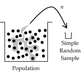
Every case in the population has the same chance of being chosen for the sample, and knowing that a particular case is in the sample provides no useful information about whether any other particular case is in the sample. The number of cases in the resulting sample is called the sample size and is denoted by n.

Simple random samples (SRS) are possible in situations where the population elements are each identified with a unique number. We can then use a random number generator to produce the sample. For example, each student enrolled in a university has a unique student number that could be used to form an SRS of students from that university.

Could we use simple random sampling to sample 14,913 undergraduates from across Canada? 

In theory, yes (append to each student number a unique university number, then randomly select 14,913 numbers), but in practice, this is not really a workable sampling scheme.

For a population like the Adams River sockeye salmon, it’s essentially impossible to collect a true SRS since the individual fish in the population don’t come with nice identifying numbers!

Stratified Random Sample

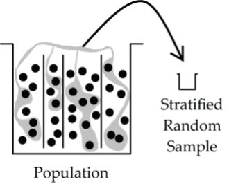
First the population is subdivided (stratified) into sub-populations called strata, and then simple random samples are drawn from each stratum.

How should the strata be created?

Ideally, we would try to choose sub-populations (strata) that are as alike as possible (homogeneous) with respect to the variable(s) of interest. For the Canadian university student example, possible strata are provinces (BC, Alberta, etc.), or year of study (1st year, 2nd year, etc.), or size of university (large, medium, or small), or program of study (Health Sciences, Business, etc.). In this example, stratifying on year of study might be the best theoretically (strata are likely more homogeneous with respect to cheating), but it would be impractical to set up an SRS from these strata across all Canadian universities. Stratifying by province or size of university is more practical.

Cluster Sample

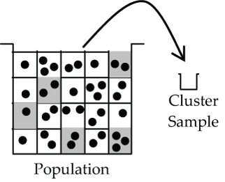
First the population is subdivided into sub-populations called clusters, and then a random sample of a few clusters is selected with every element (person) in the cluster surveyed.

How should the clusters be created?

In a sense, just the opposite of how you ideally create strata. With cluster sampling you try to create strata that are each like “mini-representatives” of the population at large. Remember, with strata the ideal was to create strata with cases that are as alike as possible. With clusters we want population-like diversity within the cluster.

For the Canadian university student example, what are possible clusters? How could we get population-like diversity within the cluster with respect to the cheating variable? Ideally, we would want students in a cluster from different programs of study, different years of study, different universities, and different regions of Canada––this type of clustering certainly doesn’t come naturally! A more natural clustering would be students in particular courses or classes within a university, but these clusters aren’t ideal for the cheating variable in the sense of population-like diversity. In practice, Canada-wide surveys are virtually never done as pure SRS, or pure stratified, or pure cluster; rather, they are done using a blended mix of these sampling schemes, which we call multistage sampling.

Multistage Sample

A multistage sample is any sampling scheme that uses a combination of simple random, stratified, and cluster sampling.

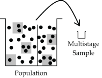
Practical realities for large populations dictate that we blend the more basic sampling schemes to form a more complicated multistage sample. For the Canadian university student example, the country could be first stratified by region (e.g., West, Prairie, Ontario, Québec, Maritimes), and then universities within each of these regions could be thought of as clusters and sampled randomly (perhaps weighted by size of university). However, not all students within a selected cluster (university) would then be sampled; rather, further stratification would first take place (e.g., year and program of study) followed by random sampling within each of these sub-strata. The random sampling of students within these sub-strata could be done by SRS or perhaps as a systematic sample (e.g., every 20th student from a student number list).

A critically important element of all the “good” sampling schemes discussed so far is that they all involve random selection at some stage. Randomization is the sampler’s best defence against sampling bias.

Systematic Sample

A systematic sample is one that is drawn systematically from some list of population elements.

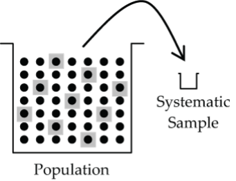
If the population elements are all nicely organized in a list (e.g., student numbers, telephone book listings), it is usually more convenient to sample them in a systematic way (say every 25^th one) than by doing an SRS. For systematic sampling to be valid, there must be no association between the order of the list and the variable(s) being investigated. If at all in doubt, don’t do a systematic sample!

For example, suppose that the Vancouver School Board wanted to assess the public’s awareness level of a new adult English as a Second Language (ESL) program. To investigate this, would it be appropriate to systematically sample every 1,000^th name in the Vancouver phone directory? Several concerns and issues arise. Firstly, what is the population of interest? Is it all adult Vancouverites? Is it all adult Vancouverites that might enrol themselves or family members in such a program? Or, is it some other population? The critical first step is to clearly identify the population of interest. Once the target population is identified, we must ensure that the sampling scheme truly draws from that population. In technical terms, the sampling frame (the list or population that you sample from) must match the population of interest.

In our example, if the population of interest is all adult Vancouverites, the phone book listing doesn’t really capture all members in the population because some adults aren’t accessible through listed phone numbers. Of course, a mismatch of sampling frame and target population is a problem for any sampling scheme, not just systematic.

Let’s forge on and accept the telephone book listing as an acceptable sampling frame. Is a systematic sample from this listing valid for this variable? Can you think of any reason that there would be an association between the alphabetical listing of names in the phone book and awareness of ESL programs? I can! Undoubtedly, awareness of ESL programs will vary according to ethnic background, and there are obvious surname groupings in the phonebook listings reflecting different ethnic backgrounds (e.g., Smith, Wong). So, a systematic sampling scheme here is unwise given the likely association between the phonebook listing and variable of interest.

Census

A census samples every element of the population.

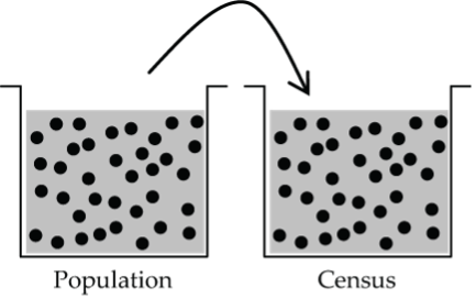
A census is a very special (and very unusual) sample that tells you everything that you want to know about a population.

Bias and Sampling

Bias is bad! Sampling error is a fact of life.

In statistics, the term bias means any sort of systematic (intentional or not) misrepresentation of the population by the sample. It is very important to distinguish between bias and sampling error. Sampling error (sampling variability) is simply sample-to-sample variation caused by the random component of a sampling scheme. While we would like to make this sampling error as small as possible (a goal of any sampling scheme), it is something that we can live with, and we can predict its size in advance. You’ve probably heard the results of a poll being qualified with a phrase like “percentages given are accurate within 3 percentage points, 19 times out of 20.” That’s an example of a particular type of sampling error that we’ll investigate in detail in Unit 3.

Possible sources of bias in sampling:

1. Bias from self-selecting or voluntary samples: Often, samples are collected through open invitation to participants broadcast over the internet, or on the radio, or in publications. This self-selecting type of sample always runs the risk of bias, because typically only those who feel strongly (for or against) respond. Seldom is any sort of statistical analysis valid for self-selecting or voluntary samples.
2. Bias from convenience samples: As the name implies, a convenience sample is one that is collected from “at hand” subjects (e.g., customers entering a store, patients admitted to a hospital). The problem with convenience samples is that there is really no way of substantiating that they are representative of some population. They may or may not be representative. If they are not, then a bias is introduced.
3. Non-response bias: Even good sampling schemes can be undermined by chosen sample members who won’t or can’t respond. These unmeasured non-responders often differ from the responders with respect to the variable of interest, and therefore, their absence biases the results.
4. Response bias: Poorly worded questions or poor interview technique can dramatically bias the response of sample members.
5. Undercoverage bias: A bias is potentially introduced if the sampling frame does not include all members of the target population. If these excluded population members differ in opinion from those in the sampling frame, a bias occurs.

How large a sample do I need for the sample to be representative?

Good question, but tough to answer in general because sample size depends on many things such as sampling scheme, parameter(s) of interest, accuracy, and confidence desired, but amazingly not the size of the population.

The sample size needed for a desired accuracy does not depend on the size of the population from which the sample is drawn (subject to some “fine-print” qualifications!).

Wait a minute, this can’t be right! Let’s take two very differently sized populations—say the population of Canada (around 35 million) vs. the roughly ten-times larger population of USA (around 317 million). Suppose that we want to estimate the percentage of pet owners in each population. Surely a sample of all 35-million Canadians (a census) will give a more accurate estimate of the percentage of pet owners in Canada, compared to a sample of only 30-million Americans for the percentage of pet owners in USA. Certainly true! Yes, population size does play a role in sample accuracy in situations where the sample size is a significant percentage of the population size (say greater than 10%).

But what if we were to randomly sample only 1,000 Canadians and 1,000 Americans? Both samples are very small relative to their population sizes. Is it still true that the Canadian estimate is more accurate?

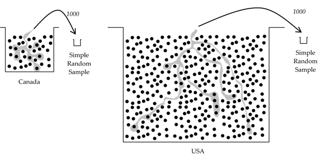
Remarkably, an estimate based on 1,000 Americans is as accurate as the estimate based on 1,000 Canadians. It’s analogous to tasting a soup––a spoonful from a well-mixed small bowl will give you just as accurate an assessment of the soup’s flavour as a spoonful from a large bowl.

If the sample size is small compared to the population size (say 10% or less), the accuracy of the sample depends on the size of the sample but not the size of the population.

Experiments

Can an experiment establish a causal relationship?

Yes—that is usually the objective of the study!

Consider the causal objective of the following research (Sridevi et al., 2006): whether plant sterols affect C-reactive protein (CRP). (Note that bold text was added to highlight key features of the research.)

And now––the key aspect of what defines an experiment––random assignment of the subjects to the treatment groups by the researchers:

In this experiment, there was one factor (variable) under study (plant sterol supplementation) with two treatment levels: Placebo Beverage (no sterol) and Sterol Beverage (1 g/240 mL).

What is a placebo?

A placebo is an inactive treatment (“sugar pill”).

If a placebo is inactive, why use it?

Subjects who are assigned to receive a placebo, or sham treatment, often show a remarkable improvement for psychological, or perhaps even physiological, reasons. We need this placebo group as a control group to compare to those receiving the active agent; otherwise, we could end up falsely concluding that the subject improvement was due to the active agent when in fact it was just the placebo effect.

Are the subjects aware that they are getting just a placebo vs. the active treatment?

Usually not. The preferred experimental design blinds the subject as well as those collecting the data in such a way that neither of them knows which treatment the subject received. This is called double blinding.

What’s the objective of double blinding?

Intentionally or not, subjects and data collectors may respond differently if they knew which treatment the subject received. Blinding removes this potential source of bias. Although the abstract for the orange juice experiment doesn’t explicitly state that double blinding was used, it likely was.

In a study such as this, it is common to compare the treatment groups on many different response variables. The response variables referred to in the Results section are total cholesterol level, LDL cholesterol level, HDL cholesterol level, triacylglycerol level, glucose level, liver function, vitamin E level, carotenoid, and CRP concentrations.

Some of the differences are judged significant, others are not––what does this mean?

When an observed difference is judged to be statistically significant, it means that subject-to-subject variation alone is unlikely to be the reason for the difference. In this abstract, the authors have abbreviated the term statistically significant to just significant. They conclude that the observed differences (Placebo vs. Plant Sterol) in total cholesterol, LDL cholesterol, HDL cholesterol, and CRP concentration are statistically significant––i.e., it is unlikely that chance variation alone accounts for the observed difference.

What do P<0.01, P<0.001, P<0.05, etc. mean?

These are probabilities called p-values that result from statistical analyses. P-values form the basis on which we judge the results as statistically significant or not. We’ll get into the specifics of statistical analyses and p-value calculations from Unit 3 on.

Based on this experiment, the authors conclude that plant sterol supplementation is effective in reducing (i.e., causes a reduction) in CRP and LDL cholesterol.

Is this conclusion limited to the 72 subjects in the study?

No, the authors are making a statistical inference that these reductions hold true for some larger (unstated) population based on the sample evidence provided by the 72 subjects.

Has the conclusion been proven with certainty?

No, it is impossible to prove with certainty inferences made about a population based on only sample evidence. Probabilistically, the sample evidence strongly suggests that plant sterol supplementation is effective in reducing CRP and LDL cholesterol. This important idea will be formalized in Unit 3.

Summary of the Four Principles of Experimental Design

1. Control aspects of the experiment that we know may have an effect on the response variables. For example, the Design section in the sterol supplementation experiment indicates that only healthy subjects were chosen. If the experiment had included subjects with health issues (e.g., high cholesterol), there likely would have been more variation in the response variables since another source (reason) for variation has been introduced (healthy vs. unhealthy subjects). This additional variation would then make it more difficult to detect differences in cholesterol levels due to the plant sterol.
2. Randomize the assignment of the subjects (experimental units) to the treatment groups to even out effects that we cannot control.
3. Replicate over as many subjects as possible. In order to make valid statistical inferences (generalizations to a population from sample evidence), we need sample information from a number of subjects (the more the better). In addition, the conclusions of an experiment are greatly strengthened if the entire experiment can be replicated elsewhere with the same results.
4. Block the subjects into similar subgroups before assigning the treatments to reduce variation in the response variables. For example, in the sterol supplementation experiment, the healthy subjects could have been blocked into age or fitness level sub-groups before randomly assigning the two treatments. This blocking then allows us to control for variation in cholesterol levels due to age or fitness level.

Next, consider the following research (Candow et al., 2006) on supplements and exercise:

What type of experimental design is this?

This is an experiment since the subjects were randomly assigned to the treatment groups.

But how was the randomization done?

If 9 of the 27 subjects were randomly assigned to each of the three treatment groups, then it would be a completely randomized design.

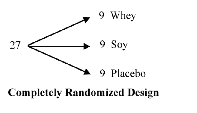
If the 27 subjects were first blocked into two sub-groups, female and male, and 6 females and 3 males were randomly assigned to each treatment, then it would be a randomized block design. Since the abstract indicates that each treatment group had 6 females and 3 males, it was likely run as a randomized block design to control for female-male variation. 

Were there any other control measures taken in the design?

Yes, only healthy, untrained subjects aged 18–35 were included. In addition, a control group (placebo) was used.

What is the factor in this experiment?

Protein supplementation.

What are the treatments?

Three treatments: whey protein, soy protein, and placebo.

What are the response variables?

Three response variables measured: lean tissue mass, strength, and indicator of myofibrillar protein catabolism.

Were any of the differences between the treatment groups found to be statistically significant?

Although these authors didn’t use the term “statistically significant” explicitly, their results showed a difference in the protein groups (whey and soy) compared to the placebo (P < 0.05 signals this, and in Unit 3 we’ll see why).

Does statistical significance mean that the difference is important in a practical sense?

Not necessarily. Statistical significance is a technical conclusion that means that the observed difference is unlikely to be the result of natural subject-to-subject variation. It could well be that the statistically significant result is quite small and of little practical importance. The authors of this study suggest in the conclusion that protein supplements produced minimal beneficial effect (even though it was statistically significant). Their knowledge of physiology allows them to judge the size of the difference in practical terms. Statistical analyses judge the size of the difference in probabilistic terms. It’s important for you to be aware of the distinction between statistical significance and practical significance. We’ll see more on this distinction from Unit 3 on.

What type of experimental design is this?

Completely randomized design. Note that only the examiner was blinded, not the patient.

Are there any control measures taken in the design?

None apparent other than subjects presumably needed their teeth bleached based on a personal assessment. Perhaps a control group using a placebo (fake bleach) should have been included to control for the placebo effect of subjects that “brushed extra hard or carefully” to come out with good results in the experiment!

What is the factor in this experiment?

Teeth bleaching frequency per day.

What are the treatments?

Two treatments: Group 1—bleach once a day, Group 2—bleach twice per day

What are the response variables?

Cromascop shade scores measured at baseline (start of experiment), and after one, two, and three weeks, as well as after one, three, six, and nine months.

Were any of the differences between the treatment groups found to be statistically significant?

Yes, there were statistically significant improvements for both treatment groups compared to their respective baseline shade scores based on a paired before/after analysis. (We’ll cover the “t-test for paired samples” in Unit 5.) Also note that the difference between the two treatment groups was judged to be not statistically significant. This means that the observed difference between the two groups wasn’t large enough to rule out natural subject-to-subject variation as the reason for the difference.

Finally, consider the following research on astronaut physiology (Cao, 2005), which illustrates a special type of blocking that is commonly used to reduce variability.

What type of experimental design is this?

A matched pair design is a special type of blocked design where “blocks” of matched pairs are first set up and then the treatment levels are randomly assigned within each matched pair. Here twin pairs are used, but in general matching is not limited to twin pairs. Two people could be matched according to some criteria that the researchers consider to be related to the variable(s) of interest in the study.

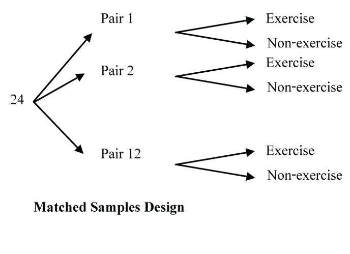
The objective of matching is the same as blocking––reduce the variability of the responses due to other factors to allow us a sharper comparison of our treatment groups.

What is the factor in this experiment?

Exercise

What are the treatments?

Exercise group, non-exercise (control) group

What are the response variables?

Lumbar spinal length, lumbar intervertebral disk heights, lumbar lordosis (abnormal forward curvature of the spine)

Were any of the differences between the treatment groups found to be statistically significant?

Yes, the Results section identifies several statistically significant increases and decreases.

Long Descriptions

• Figure 1: Diagram showing a population being represented as a large bucket with a sample being a small cup from that bucket. Three different population “buckets” are shown – “Canadian University Students”, “Adams River Sockeye”, “Cars produced in a given year”. Each bucket shows a small cup being taken from bucket which is the sample. [Back to Figure 1]
• Figure 2: Diagram showing a population bucket with members of population represented by randomly scattered dots within bucket. A selection of six random dots is shown within a grey coloured area which is pointed towards the small sample cup. The number of samples is labelled as “n” and this type of sample is labelled as a “Simple Random Sample” [Back to Figure 2]
• Figure 3: Diagram showing a population bucket with members of population represented by randomly scattered dots within bucket. There are three vertical lines splitting the population into four groups. A random sample is shown being selected in each group using shading. The selected dots are pulled from the population to create a sample which is labelled a “Stratified Random Sample”. [Back to Figure 3]
• Figure 4: Diagram showing a population bucket split up into a grid with varying numbers of the population in each grid cell. Four grid cells are shown shaded and being added to sample which is labelled “Cluster Sample”. [Back to Figure 4]
• Figure 5: Diagram showing a population bucket with a vertical line to split population into two larger groups. Population dots are clustered and a subset of clusters is drawn from each group to be combined into a Multistage sample. [Back to Figure 5]
• Figure 6: Diagram which shows a population bucket with an ordered grid of dots. Starting from the left most side every fifth dot is selected to be part of sample. This type of sample is called a Systematic Sample. [Back to Figure 6]
• Figure 7: This diagram illustrates what a census. A population bucket with random dots representing the population all selected is drawn. A second bucket of same size is drawn beside. All population dots are selected to be in the second bucket. This second bucket represents a census. [Back to Figure 7]
• Figure 8: Diagram illustrating a sample of 1000 people from the population of Canada and 1000 people from the population of the United States. Canada with the smaller population is represented by a smaller bucket and the United States with a much larger population is represented by a bucket that is over 5 times of large. A thousand people are sampled from each in using the Simple Random Sample technique. [Back to Figure 8]

References

Andersen, L., Jacobs, D., Carlsen, M., & Blomhoff, R. (2006). Consumption of coffee is associated with reduced risk of death attributed to inflammatory and cardiovascular diseases in the Iowa Women’s Health Study. American Journal of Clinical Nutrition, 83(5), 1039–1046. https://doi.org/10.1093/ajcn/83.5.1039

Candow, D. G., Burke, N. C., Smith-Palmer, T., & Burke, D. G. (2006). Effect of whey and soy protein supplementation combined with resistance training in young adults. International Journal of Sport Nutrition and Exercise Metabolism, 16(3), 233–244. DOI: 10.1123/ijsnem.16.3.233

Cao, P. (2005). Exercise Within Lower Body Negative Pressure Partially Counteracts Lumbar Spine Deconditioning Associated With 28-day Bed Rest. Journal of Applied Physiology, 99(1), 39-44. https://doi.org/10.1152/japplphysiol.01400.2004

Celia Hall. (May 12, 2006 Friday). Imagine that — coffee’s good for you: Study, which followed 27,000 older women for 15 years, found a 30-per-cent reduced risk of cardiovascular disease in those people who had a moderate intake of the beverage. The Vancouver Sun (British Columbia). https://advance.lexis.com/api/document?collection=news&id=urn:contentItem:4JXX-4VC0-TWD4-02CW-00000-00&context=1516831

Devaraj, S., Autret, B. C., and Jialal, I. (2006). Reduced-calorie orange juice beverage with plant sterols lowers C-reactive protein concentrations and improves the lipid profile in human volunteers. (2006). American Journal of Clinical Nutrition, 84(4), 756–761. https://doi.org/10.1093/ajcn/84.4.756

Herring, J. (2021, May 29). Academic cheating skyrockets during pandemic: UCalgary researcher [Adapted]. Calgary Herald https://calgaryherald.com/news/local-news/academic-cheating-skyrockets-during-pandemic-ucalgary-researcher

Zantner, C., Derdilopoulou, F., Martus, P., & Kielbassa, A. M. (2006). Randomized clinical trial on the efficacy of a new bleaching lacquer for self-application. Operative Dentistry, 31(3), 308–316. https://doi.org/10.2341/05-69