Supplementary Notes 3.1

Sampling Variability

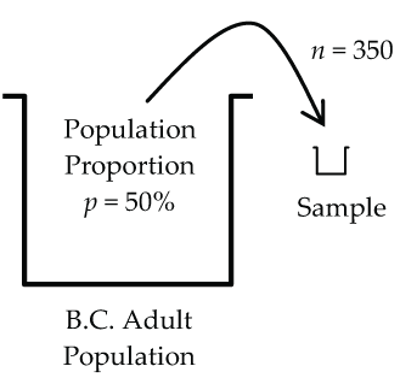
In this survey, Ipsos randomly sampled 350 adult British Columbians and discovered that 175 of them (50%) said that their local environment was getting worse. This 50% is a sample proportion calculated from the responses of the 350 people selected in this particular random sample.

If Ipsos took another random sample of 350 British Columbians, it might find that 182 (52%) say that their local environment is getting worse. With yet again another random sample of 350, it might find that only 161 (46%) say that their local environment is getting worse … and so on with each random sample of 350 people producing a slightly different sample proportion.

The point is that the sample proportion fluctuates somewhat from sample to sample depending on which 350 British Columbians are actually selected. That’s why Ipsos includes a “±5.2 percentage points, 19 times out of 20” margin of error statement.

In Lesson 3.2, we will cover in detail the specifics of this margin of error calculation and interpretation for sample proportions. Before we can tackle these specifics, we need to answer fundamental questions: As the sample proportion fluctuates from sample to sample, what pattern does it follow, where is it centred, and how much variability does it have? To gain some insight into the answers to these questions, let’s do a simulation.

Simulating the Sampling Distribution of a Proportion

Suppose that 50% of the BC adult population think that the quality of the environment is getting worse. Simulating on the computer, we are going to repeatedly sample 350 adults from this population, and for each sample, record the sample proportion of people who think the environment is getting worse.

Normal Model for the Sampling Distribution of a Proportion

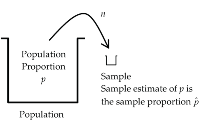
We can use this simulation to get a feel for how a sample proportion, , fluctuates from sample to sample. Of course, if we take only one sample, is just a single number calculated from the data. But if we visualize taking all possible samples, fluctuates according to some distribution called the sampling distribution for . Later on, we’ll use this sampling distribution for  to judge whether a particular  in one sample is unusual.

In general, the exact sampling distribution for is very complex, but under some reasonable conditions, we can approximate it quite accurately with a normal model.

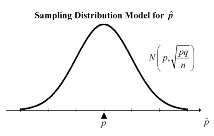
For large independent samples, the central limit theorem (CLT) says that the sampling distribution of the sample proportion, , can be approximated by a normal model with mean, , and standard deviation, , where .

The standard deviation of a sample estimate based on its sampling distribution is called the standard error of the estimate. So, in this case, we say the standard error of the sample proportion is .

In a typical statistical application, the population proportion, , is unknown, and we take a random sample to estimate . Then the estimated standard error of the sample proportion is .

Before the sample is actually collected, visualize the sample estimate, , as a variable “floating” around according to this normal model. The normal model tells us that, on average, the estimate will hit the target, , and it will typically deviate from by a standard deviation given by (which will be very small for large sample sizes ).

Technical Conditions

1. The sampled values must be independent of each other.

   Independence Condition

   For example, this will be the case if the observations are from a simple random sample.

2. The sample size, , is large enough.

   Success/Failure Condition

   The working guideline for how large is large enough is and . This ensures that the tail of the normal model for doesn’t cut off a meaningful amount of probability below 0 or above 1, which are impossible values for the sample proportion, .

3. The sample size is no larger than 10% of the population.

   10% Condition

   This will be the case if we randomly sample observations from a very large population and is less than 10% of the population size.

Example 1: Normal Model for the Sampling Distribution of a Proportion

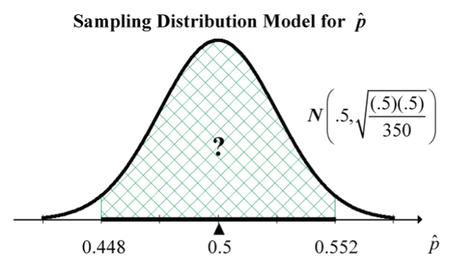
Suppose that 50% of the entire BC adult population thinks that the quality of the environment is getting worse. Here, we’re proposing a specific value for a population proportion: .

Now imagine taking a random sample of 350 adults from the BC adult population and calculating the sample proportion, , that say the environmental quality is getting worse.

What is the probability that this sample proportion will fall between 44.8% and 55.2%?

Normal Model Condition Check

• Independence: The sample is random, so it’s reasonable to assume that our sampled values are independent of each other.
• Success/Failure Condition: Here, and .
• 10% Condition: Our sample of 350 is far less than 10% of the BC adult population.

Since all three conditions are satisfied, it is reasonable to use the normal model for the sampling distribution of .

The Probability Calculation

Recall from Supplementary Notes 2.3 how to do probability calculations in R. Here, the code, pnorm(0.552, mean=0.5, sd=sqrt(0.5*0.5/350)) - pnorm(0.448, mean=0.5, sd=sqrt(0.5*0.5/350)) returns the answer of 0.9483. So, there is about a 95% (94.83%) chance that the sample proportion will fall between 44.8% and 55.2%.

Discussion

The Ipsos poll results claimed that a random sample of 350 adult British Columbians had a margin of error of ±5.2 percentage points, “19 times out of 20” (Ipsos, 2006). We’ve just shown that if the true population proportion is 50%, then the sample proportion has a 95% chance of being between 44.8% and 55.2%. Said another way, there is a 19 times in 20 chance that the sample proportion is between 44.8% and 55.2%; i.e., within ±5.2 percentage points of the true value of (50% in this case).

It’s still premature to say exactly what we mean by margin of error, but the probability calculation done in this question certainly seems to confirm the Ipsos claim.

Example 2: Normal Model for the Sampling Distribution of a Proportion

Is it unusual for a “6” to come up 60 or more times in 300 rolls of a die?

If the die is fair, we expect a 6 to come up one-sixth of the time. Here, we’re proposing a specific value for a population proportion: .

So, in 300 rolls, we expect to roll a 6 about 300(1/6) = 50 times. So, getting 60 or more 6s is definitely more than expected. Let’s answer the question of how unusual this is by calculating the probability of getting 60 or more 6s in 300 rolls of a fair die. In terms of proportions, we want to calculate the chance that the proportion of 6s in 300 rolls is 60/300 = 0.2 or more; i.e., find .

First, we will check the appropriateness of using the Normal model.

Normal Model Condition Check

• Independence Condition: We know that with a fair die, the outcome on each roll is independent of what happens on any other roll.
• Success/Failure Condition: Here and .
• 10% Condition: The population size here is infinite because the die can be rolled forever.

Since all three conditions are satisfied, it is reasonable to use the normal model for the sampling distribution of .

The Probability Calculation

In R, the code, 1 - pnorm(0.2, mean=1/6, sd=sqrt((1/6)* (5/6)/300)) returns the answer of 0.06067. So, there is about a 6% chance of getting 60 or more 6s in 300 rolls of a fair die. This is somewhat unusual, but not exceptionally unusual.

Another way to judge unusualness is to answer the question: How many SDs is 60 6s in 300 rolls above the expected 50?

Phrasing this question in terms of proportions, it becomes: How many SDs is 60/300 = 0.2 above the expected 1/6? Here .

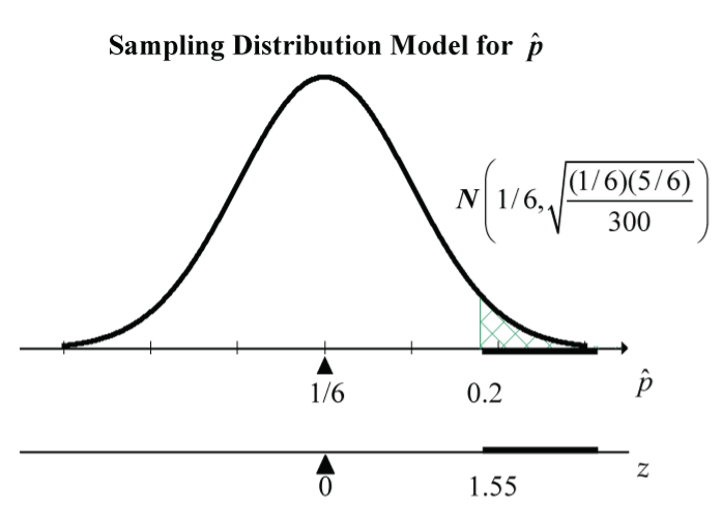
So, 0.2 is SDs above the expected 1/6.

Discussion

This is somewhat unusual, but not exceptionally unusual.

Example 3: Normal Model for the Sampling Distribution of a Proportion

Suppose an airline has 210 seats available for a flight, and that it knows that, on average, 10% of its customers making an advance booking end-up cancelling. Here, we’re proposing a specific value for a population proportion .

If the airline accepts 225 advance bookings, what is the chance that the flight will be oversold, and some passengers will have to be bumped from the flight?

In this question, the connection with sample proportions is not obvious, so as a first step, let’s see if we can re-express the question into one involving a sample proportion.

We want: P(flight oversold). The flight is oversold if more than 210 passengers show up. This happens if there are fewer than cancellations; i.e., cancellations. So, if the proportion of cancellations is (about 6%), the flight is oversold.

So, P(flight oversold) = P(), where is the proportion of cancellations in a sample of 225.

OK, now we’re ready to proceed with the normal model check.

Normal Model Condition Check

• Independence Condition: Is it reasonable to assume that passenger cancellations are independent of each other? There is certainly some doubt here since cancellations could occur in bunches due to related people travelling in family or business groups.
• Success/Failure Condition: Here, and .
• 10% Condition: The population of people potentially making airline bookings is unknown, but certainly it is large enough to assume that n = 225 is less than 10% of it.

We have flagged the independent observations condition as a concern, but we’ll continue the calculation assuming that cancellations are independent of each other and that the normal model is appropriate.

The Probability Calculation

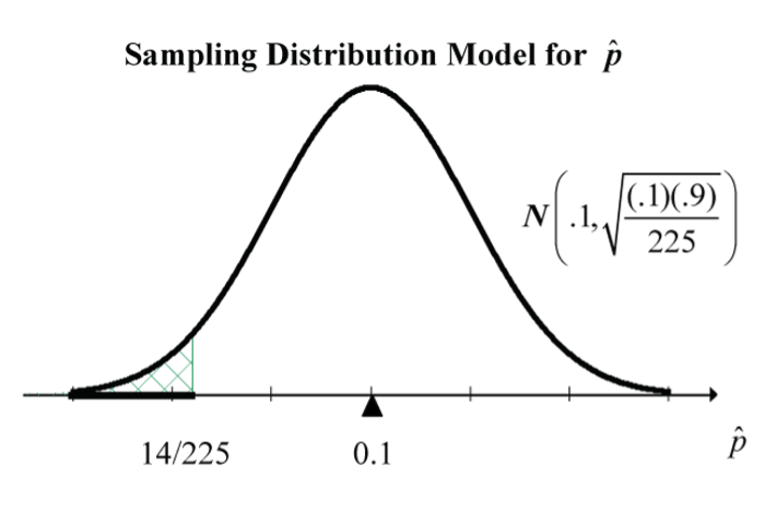
In R, the code, pnorm(14/225, mean=0.1, sd=sqrt(0.1*0.9/225)) returns the answer of 0.02945.

Discussion

So, there is only about a 3% chance that the flight will be oversold (assuming that passengers cancel independently of each other).

References

Ipsos. (2006, October 18). Ipsos quick poll on environmental issues. Retrieved from http://www.ipsos-na.com/news-polls/pressrelease.aspx?id=3225