Lesson 3.3: Hypothesis Testing
Supplementary Notes 3.3
Hypothesis Test for a Proportion
Introduction: The Statistical Courtroom
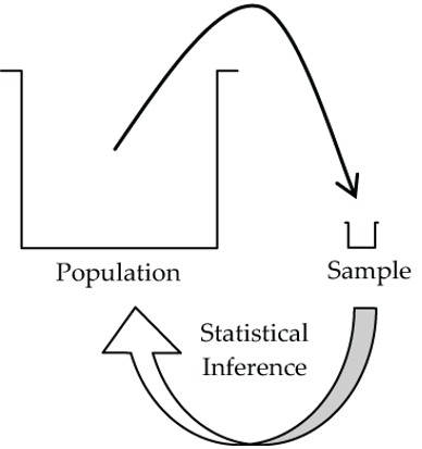
Generalizing about the population based on sample results, that’s what statistical inference is all about.
In Lesson 3.2, we “generalized” the sample proportion to construct a confidence interval that was designed to contain the population proportion with a high degree of confidence. In this lesson, we will generalize the sample proportion to test hypotheses (claims) about the corresponding population proportion.
Testing hypotheses is one of the most extensive application areas in all inferential statistics. In fact, all the remaining topics in this course focus on testing hypotheses in various experimental settings.
No matter what the experimental setting is, all hypothesis tests have a common structure that is analogous to a courtroom trial. In statistics, we put a hypothesis, called the null hypothesis, on “trial.” Evidence in the form of sample data is presented against the null hypothesis. If the evidence is strong enough against the null hypothesis, we find it “guilty,” and our “verdict” is to cast the null hypothesis aside, or reject it, in favour of “not-the-null-hypothesis.” Rather than call it “not-the-null-hypothesis,” statisticians call this competing hypothesis the alternative hypothesis. If, however, the sample evidence is not strong enough to reject the null hypothesis, we conclude that the null is “not guilty” and fail to reject it. Failing to reject the null certainly doesn’t prove it true, or even imply that our sample evidence supports it, just that the evidence is not strong enough to reject it.
The essential distinction between the null and alternative hypotheses in a statistical test is that the null hypothesis is the “weak” hypothesis, and the alternative hypothesis is the “strong” hypothesis. The alternative is strong in the sense that the statistical test will conclude the alternative only if the data evidence is strongly against the null in favour of the alternative. The null hypothesis is weak in the sense that the statistical test will default to it anytime that the data evidence is not strongly against it. It gets the name “null” for a reason: It’s the “know nothing” or “status quo” hypothesis.
The statistical version of the courtroom trial has one huge advantage over the real thing. Through a probability calculation called a p-value, the statistical test can objectively measure just how unlikely the sample evidence is under the null hypothesis model. Of course, no such objective measure is available to a real jury in the courtroom. The p-value calculation is based on a sampling distribution model for the particular statistical test being applied.
Before we plunge into the details of testing a proportion, let’s walk through a typical research study and highlight the key components of a statistical test.
Example: A Typical Hypothesis Test from Recent Research
For this example, we will read from the abstract of a research study.
Effect of Low-Repetition Jump Training on Bone Mineral Density in Young Women
Adapted from Kato, T., Tersashima, T., Yamashita, T., Hatanaka, Y., Honda, A., & Umemura, Y. (2005). Effect of low-repetition jump training on bone mineral density in young women. Journal of Applied Physiology, 100(3), 839–843. doi: 10.1152/japplphysiol.00666.2005. Used with permission.
Aims: The hypothesis of the present study was that low-repetition and high-impact training of 10 maximum vertical jumps/day, 3 times/week would be effective for improving bone mineral density (BMD) in ordinary young women.
Methods: Thirty-six female college students, with mean age, height, and weight of 20.7+/-0.7 yr, 158.9+/-4.6 cm, and 50.4+/-5.5 kg, respectively, were randomly divided into two groups: jump training and a control group.
Results: After the 6 months of maximum vertical jumping exercise intervention, BMD in the femoral neck region significantly increased in the jump group from the baseline (0.984+/-0.081 vs. 1.010+/-0.080 mg/cm2; P<0.01), although there was no significant change in the control group (0.985+/-0.0143 vs. 0.974+/-0.134 mg/cm2). And also lumbar spine (L2-4) BMD significantly increased in the jump training group from the baseline (0.991+/-0.115 vs. 1.015+/-0.113 mg/cm2; P<0.01), whereas no significant change was observed in the control group (1.007+/-0.113 vs. 1.013+/-0.110 mg/cm2).
Conclusion: From the results of the present study, low-repetition and high-impact jumps enhanced BMD at the specific bone sites in young women who had almost reached the age of peak bone mass.
Which hypothesis do you think the authors are stating in the Aims section: the null or the alternative?
How was this study conducted?
From the Methods section, we know this study was conducted as a one-factor (type of training program) completely randomized experiment with two treatment levels (jump training, control).
In the Results section, “significantly increased” means that a statistical test determined that the observed increases in BMD from baseline (i.e., start of the study) for the jump group were very unlikely to be due to natural subject-to-subject variation occurring under a null hypothesis model. How unlikely?
The rejection of the null hypothesis allows the authors to reach the strong conclusion of the alternative hypothesis: Jump training enhances BMD in young women.
Example: Motivate the One-Proportion Z-Test
The objective of this example is to introduce the main ideas of a particular hypothesis test, called the one-proportion Z-test, that will be the focus for the remainder of this section.
A municipality is considering the acquisition of new parkland. Since there is considerable cost in purchasing the new parkland, the municipality wants reassurance that more than 50% of its voters support the acquisition.
The first, all-important step in any testing hypotheses application is to correctly identify the null and alternative hypotheses. Notice that in this application, the municipality wants reassurance that more than 50% support the purchase, so that would be the strong conclusion, and consequently, “more than 50% support the purchase” is the alternative hypothesis. The null (fall-back) hypothesis is that 50% support the acquisition. Symbolically we write:
- Null Hypothesis: H0: p = 50%
- Alternative Hypothesis: HA: p > 50%
where p is the population proportion that supports the purchase.
To investigate the level of voter support on the acquisition, the municipality plans to randomly sample 100 voters and base its decision on the sample proportion,  , that are in favour of the purchase.
If you were the statistical consultant for the municipality, what would you recommend for each of the following scenarios for the sample proportion?
- = 45/100 = 45%: A 45% sample proportion certainly is not strong evidence that more than 50% of the voters support the purchase, i.e., that p > 50%, so do not reject the null hypothesis. Do not recommend purchase of the new parkland.
- = 50/100 = 50%: A 50% sample proportion suggests that p is around 50%, but remember you need strong evidence before recommending the purchase. This is not strong enough to conclude with any confidence that p > 50%, so do not reject the null hypothesis. Do not recommend purchase of the new parkland.
- = 55/100 = 55%: A 55% sample proportion makes the recommendation more difficult. The sample evidence is certainly in the direction of the alternative hypothesis, but is it strong enough? Let’s look at it this way: If only 50% support the purchase (p = 50% and H0 is true), the sampling distribution for will follow a normal model centred at 50% with an SD of √((0.5×0.5)/100) = 0.05 = 5%. With this model, 55% is only 1 SD above the mean and would not be considered particularly unusual. Consequently, the sample evidence is not strongly supporting p > 50%, so do not reject the null hypothesis. Do not recommend purchase of the new parkland.
- = 60/100 = 60%: A 60% sample proportion is 2 SDs above the mean under the “p = 50% normal model” for the null hypothesis and would be considered an unusual outcome under this model. Most people would consider this strong enough evidence to reject the null in favour of the alternative. Recommend the purchase of the parkland!
- = 65/100 = 65%: A 65% sample proportion is 3 SDs above the mean under the “p = 50% normal model” for the null hypothesis. Very unusual. Reject the null in favour of the alternative. Recommend the purchase of the parkland!
The Four-Step Structure of a One-Proportion Z-Test
- Hypotheses
Usually, the objective of the study or research identifies the strong hypothesis, which then leads you to the setup of HA. In the context of a one-proportion population, the possible choices for this alternative hypothesis are:- HA: proportion p is greater than some specified proportion p0, i.e., p > p0
- HA: proportion p is less than some specified proportion p0, i.e., p < p0
- HA: proportion p is different from some specified proportion p0, i.e., p ≠ p0
The null hypothesis for each of these alternatives is p = p0, so in the one-proportion experimental context, we will be testing one of the following three possibilities:
- H0: p = p0 versus HA: p > p0 (upper-sided alternative)
- H0: p = p0 versus HA: p < p0 (lower-sided alternative)
- H0: p = p0 versus HA: p ≠ p0 (two-sided alternative)
- Model
We put H0 “on trial” and give it the benefit of the doubt (“innocent until proven guilty”). Consequently, we use a normal model for the sampling distribution of that has a mean of  and a SD of
  , where
  . Note: we use here, not
  .
.
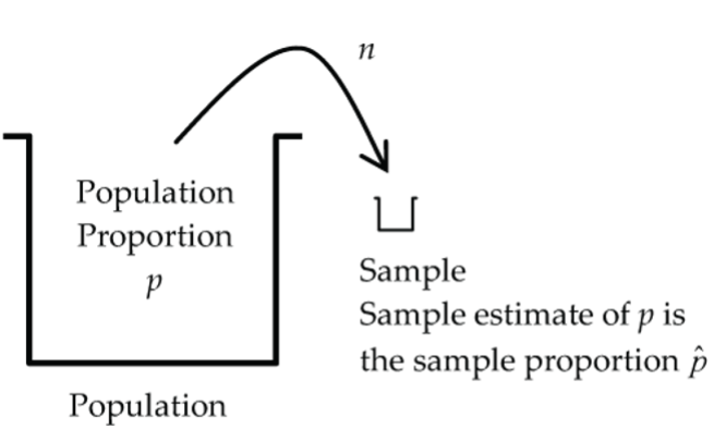
Figure 2: The sample estimate of a population (p) is the sample proportion. Assumptions: Similar to the confidence interval for the proportion p.
- Independent sample
- Random sample
- Success/failure condition (calculated using and
 , not and
  )
) - 10% condition
- Mechanics
Under the H0 model, we calculate the number of SDs that is from the null hypothesis mean of p0 using  . (This quantity is called the test statistic.)
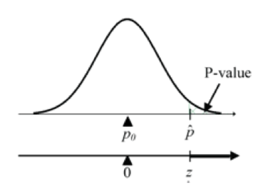
Figure 3: Upper-sided proportion test assesses if the sample results are compatible with H0 or HA models Then we use the standard normal model to calculate the p-value for this Z-statistic. This will give us a probability measure of how unusual this Z-statistic is under the H0 model. Examples of this Z-statistic calculation are presented below.
- Conclusion
A “small” p-value tells us that the observed sample results are not compatible with the H0 model, and so we reject H0 in favour of HA. On the other hand, if the p-value is not “small,” we conclude that the sample results are compatible with the H0 model, and so we do not reject H0.
P-Value Calculation for One-Proportion Z-Test
Brace yourself! The general definition of a p-value is coming-up! It may take many re-reads of this definition plus numerous examples where you see a p-value in action before you become comfortable with it.
P-Value Definition
The p-value of a statistical test is the probability under the null hypothesis model of getting a test statistic value as extreme (or more so in the direction of the alternative hypothesis) as the one that we actually got.
Let’s get specific and see how this p-value is calculated for a one-proportion Z-test.
- Upper-sided alternative:
H0: p = p0 versus HA: p > p0
Calculate test statistic:
Figure 4: Upper-sided proportion test R code:
1 - pnorm(Z, mean=0, sd=1) - Lower-sided alternative:
H0: p = p0 versus HA: p < p0
Calculate test statistic:
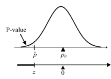
Figure 5: Lower-sided proportion test R code:
pnorm(Z, mean=0, sd=1) - Two-sided alternative:
H0: p = p0 versus HA: p ≠ p0
Calculate test statistic:
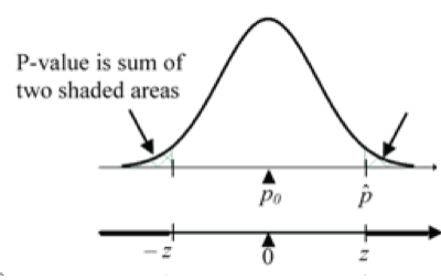
Figure 6: P-value is the sum of the two shaded areas. R code:
2 * (1 - pnorm(z, mean=0, sd=1))
Example 1: One-Proportion Z-Test
Let’s return to the example where the municipality is considering the acquisition of new parkland. Suppose that in the random sample of 100 voters, 59 were in favour of the parkland purchase. Is this sufficiently strong evidence to conclude that more than 50% of the municipality’s voters support the purchase of the parkland?
- Hypotheses
H0: p = 0.50 (50%) versus HA: p > 0.50
where p is the proportion of all voters in the municipality that support the parkland purchase. - Model
First check the conditions needed for the normal model in the one-proportion context.- Independence: Yes, individuals likely responded independently in this random sample.
- Random: Yes, a random sample was taken.
- Success/failure condition: Yes, np0 = 100(0.50) = 50 ≥ 10 and nq0 = 100(0.50) = 50 ≥ 10.
- 10% condition: Yes, n = 100 is less than 10% of a BC municipal voter population.
Because the conditions are satisfied, it is reasonable to use a normal model for the sampling distribution of
, and we can proceed with the one-proportion Z-test. - Mechanics
Calculate.
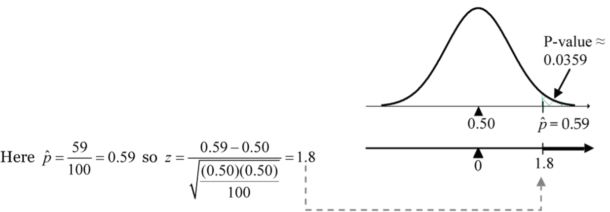
Figure 7: Proportion test assesses whether or not a sample from the population represents the true proportion of the entire population. 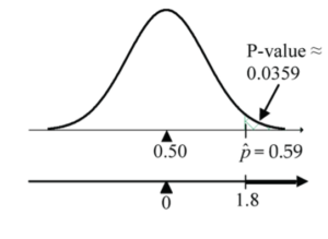
Figure 7: Proportion test assesses whether or not a sample from the population represents the true proportion of the entire population. new P-value =
1 - pnorm(1.8, mean=0, sd=1)≈ 0.0359.
A p-value of 0.0359 means that if only 50% of the voters in the population favoured the purchase (i.e., H0 is true), there is only a 3.59% chance of observing a sample proportion as large as or larger than 59%, or equivalently of observing a test statistic result as large as or larger than Z = 1.8. - Conclusion
Although there is no hard-and-fast rule as to when a p-value is small enough to reject H0, often 0.05 is used as a cutoff value. Here we have p-value = 0.0359, which is less than 0.05 and would likely be considered as small enough to reject H0 in favour of the alternative hypothesis. Consequently, the sample evidence is sufficiently strong to conclude that more than 50% of the voter population in the municipality favours the parkland purchase.
Example 2: One-Proportion Z-Test
Historically, the Green Party of Canada has been supported by 4.5% of the electorate. In a recent random sample of 800 Canadian voters, 54 expressed support for the Greens. Is this sufficient evidence to conclude that support for the Greens has changed?
- Hypotheses
H0: p = 0.045 (4.5%) versus HA: p ≠ 0.045
where p is the proportion of all Canadian voters that support the Greens.
A two-sided alternative was chosen because the question asked if the support has “changed,” and two-sided allows for the possibility that the support has gone up or down. - Model
First check the conditions needed for the normal model in the one-proportion context.- Independence: Yes, individuals likely responded independently in this random sample.
- Random: Yes, a random sample was taken.
- Success/failure condition: Yes, np0 = 800(0.045) = 36 ≥ 10 and nq0 = 800(0.855) = 764 ≥ 10.
- 10% condition: Yes, n = 800 is less than 10% of the Canadian electorate.
Because the conditions are satisfied, it is reasonable to use a normal model for the sampling distribution of
, and we can proceed with the one-proportion Z-test. - Mechanics
Calculate.
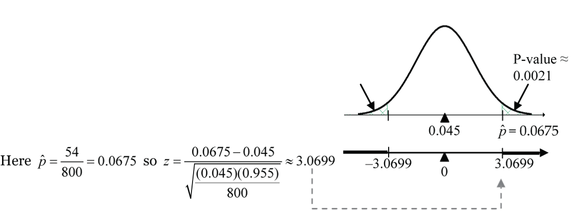
Figure 8: Proportion test 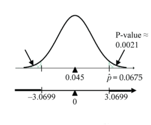
Figure 8: Proportion test new P-value =
2 * (1 - pnorm(3.0699, mean=0, sd=1))≈ 0.0021. (Note the upper-tail area is doubled because of the two-sided alternative hypothesis.)
A p-value of 0.0021 means that if in fact only 4.5% of the voters in the population support the Greens (i.e., H0 true), there is only about a 0.2% chance (that’s only 1/5 of 1% chance) of observing a test statistic result above Z = 3.0699 or below –3.0699. - Conclusion
With such a small p-value, we would reject the null hypothesis in favour of the alternative hypothesis. The sample provides sufficient evidence that support for the Green Party has changed from the historical 4.5%; in fact, we can now say that it has increased from 4.5%. How much? Well, a 95% CI for the proportion supporting the Greens is , which gives 0.0675 ± 0.0174 or between 5% and 8.5%.
Example 3: One-Proportion Z-Test
A drug detection device is tested on a series of five packages, only one of which contains drugs. The device correctly identifies the package with drugs in 115 out of 500 independent trials. Is this sufficiently strong evidence to conclude that the device does better than chance at detecting the drug package?
- Hypotheses
H0: p = 1/5 = 0.20 (20%) versus HA: p > 0.20
where p is the true (population) proportion of the time that the device can detect the drug package. - Model
First check the conditions needed for the normal model in the one-proportion context.- Independence: Yes, the question stipulates independent trials.
- Random: Not stated, but reasonable to view trials as a random sample.
- Success/failure condition: Yes, np0 = 500(0.20) = 100 ≥ 10 and nq0 = 500(0.80) = 400 ≥ 10.
- 10% condition: Yes, since, theoretically, the population is infinite.
Because the conditions are satisfied, it is reasonable to use a normal model for the sampling distribution of
, and we can proceed with the one-proportion Z-test. - Mechanics
Calculate.
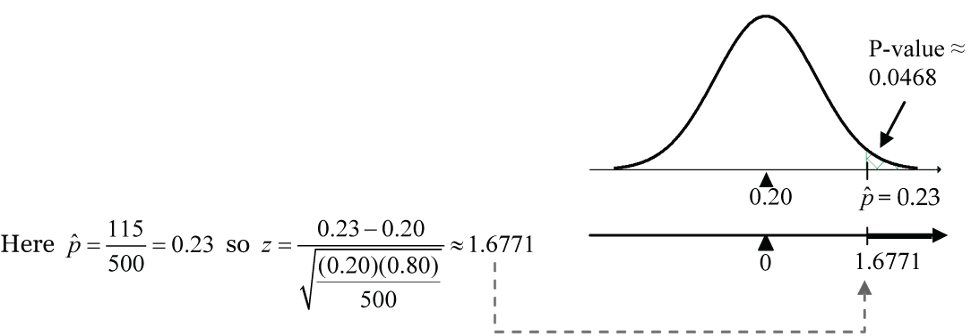
Figure 9: Proportion test 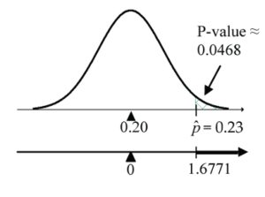
Figure 9: Proportion test new P-value =
1 - pnorm(1.6771, mean=0, sd=1)≈ 0.0468.
A p-value of 0.0468 means that if the detection rate for the device is 20% (i.e., the chance rate under H0), there is only a 4.68% chance of observing a sample proportion as large as or larger than 23%, or equivalently of observing a test statistic result as large as or larger than Z = 1.6771. - Conclusion
Our p-value of 0.0468 is less than the 0.05 cut-off that is often taken for judging statistical significance. Using this 0.05 cut-off, we reject H0 and conclude that the difference between the observed 23% detection rate and the chance detection rate of 20% is statistically significant at the 0.05 level of significance.
Level of Significance (Alpha Level)
We have already noted that there is no magical cut-off point for p-values. However, certain small probabilities like 0.10, 0.05, 0.01, and 0.001 are commonly used. If we do use a particular p-value cut-off, it is called the significance level, or alpha ( ) level, of the test.
Significance Level |
Reject H0 at Significance Level α If |
| α = 0.10 | P-value < 0.10 |
| α = 0.05 | P-value < 0.05 |
| α = 0.01 | P-value < 0.01 |
| α = 0.001 | P-value < 0.001 |
How do we know which significance level to choose?
There is no hard and fast rule, but there are considerations and consequences that can serve as guidelines for choosing the level at which we declare statistical significance. Remember that the p-value is the probability that we calculate under the null hypothesis model to judge the unusualness of our sample results against this model.
- If we set the p-value cut-off high (say 0.10), then we run a higher risk of falsely rejecting H0 than if we set the p-value low (say 0.001). Setting the p-value high might make sense in pilot studies where researchers are just beginning their search for possible relationships, which will be confirmed with more extensive follow-up studies using lower significance levels.
- Setting the significance level low makes it “harder” for the statistical test to reject H0, which in turn means that important departures from H0 may be missed.
Later in this section, we’ll discuss this further when we investigate Type 1 and 2 errors and the power of a statistical test.
For this course, you can use = 0.05 as the cut-off for declaring statistical significance, but realize that in practice it is not a black-and-white issue where a p-value of 0.049 is judged statistically significant, whereas 0.051 is not.
If we’re using = 0.05, then we reject H0 in favour of HA if the p-value is less than 0.05, and we fail to reject H0 if the p-value is greater than 0.05. However, what do we do if the p-value equals 0.05?
In theory, the p-value cannot be exactly equal to 0.05 since it is a continuous value. However, in practice it could depend on how much it is rounded. If that were to happen (although this is very unlikely), we are in that grey zone where it’s unclear whether or not to reject the H0. For practical purposes, we can try to find the p-value to a sufficient accuracy that it is either less than or greater than 0.05. If that is not possible, then we have to simply acknowledge that we’re in the grey zone!
Statistical Significance Versus Practical Significance
Statistical significance is a technical conclusion that results from a statistical test producing a small p-value (meaning that it’s unusual to see sample results this extreme under the null model). However, statistical significance may, or may not, have importance or significance in a practical sense.
Practical significance is a decision based on experience, or personal judgement, that a result has meaningful or important consequences in a practical sense.
Example: Statistical Significance Versus Practical Significance
This example explores the effect of sample size on statistical and practical significance. In each of the two scenarios below, we are testing H0: p = 1/5 = 0.20 (20%) versus HA: p > 0.20, where p is the true (population) proportion of the time that the device can detect the drug package.
- Suppose in our drug detection study there are 10,250 detections in 50,000 trials.
- Is this statistically significant at the = 0.01 level?
Here,
 so
so  .
.
If the sample size n is large, the variability of is small, which in turn inflates the difference between and in the numerator.
P-value =1 - pnorm(2.7951, mean=0, sd=1)≈ 0.0026 < 0.01 so reject H0.
Yes, the result is statistically significant at the = 0.01 level. A large sample is able to detect small departures from the H0 model and find them statistically significant. - Do you think this result would be judged practically significant?
Only an expert in the field could say for sure, but it seems unlikely given that the sample detection rate of 20.5% is only half of one percent above the chance rate of 20%. Based on this sample, a 99% CI for p is 20.035% to 20.965%, so even at the upper bound of 20.965, the detection rate is less than 1% above the chance model.
- Is this statistically significant at the
- Suppose in our drug detection study there are 16 detections in 50 trials.
- Is this statistically significant at the = 0.01 level?
Here,
 so
so  .
.
P-value =1 - pnorm(2.1213, mean=0, sd=1)≈ 0.0169 > 0.01 so fail to reject H0.
The result is not statistically significant at the = 0.01 level (but it’s close!).
If the sample size n is small, the variability of is large, which in turn dampens the difference between and in the numerator.
A small sample is able to detect only very extreme departures from the H0 model as statistically significant. - Do you think this result would be judged practically significant?
Given that we can’t rule out the possibility that the detection rate is no better than chance (20%), it would be highly speculative (and unwise) to declare the results to be practically significant based on this sample alone. However, with a 32% sample detection rate, the results certainly look promising and suggest the need for a larger follow-up study.
- Is this statistically significant at the
Types of Error in Testing Hypotheses
When we do a hypothesis test, we hope to reach a correct conclusion. However, since our conclusion is based on sample evidence (not the entire population), there is always the possibility that we reach a wrong conclusion and make an error. The tables below (Fig. 10) illustrate the two types of errors that are possible and show the analogy to a courtroom trial.
Statistical Test of H0
| True State
H0 True |
True State
H0 False |
|
| Statistical Decision
Reject H0 |
Type I Error | Correct Decision |
| Statistical Decision
Fail to Reject H0 |
Correct Decision | Type II Error |
Put H0 “On Trial”
Courtroom Trial
| True State
Innocent |
True State
Guilty |
|
| Jury Decision
Accused Guilty |
Error 1 | Correct Decision |
| Jury Decision
Accused Not Guilty |
Correct Decision | Error 2 |
Put Accused “On Trial”
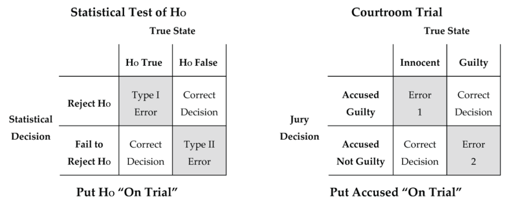
- Type 1 error: The mistake of rejecting H0 when H0 is in fact true.
- Type 2 error: The mistake of failing to reject H0 when H0 is in fact false.
Are the consequences of each type of error the same in the courtroom setting?
No, our society regards a Type 1 error (finding an innocent defendant guilty) as being more serious, and our legal system guards against it by demanding that the evidence against the accused be “beyond a reasonable doubt” before the jury finds an accused guilty.
Are the consequences of each type of error the same in the hypothesis testing setting?
Probability of Type 1 and 2 Errors
The previously discussed significance level can now also be interpreted as the probability of a Type 1 error.
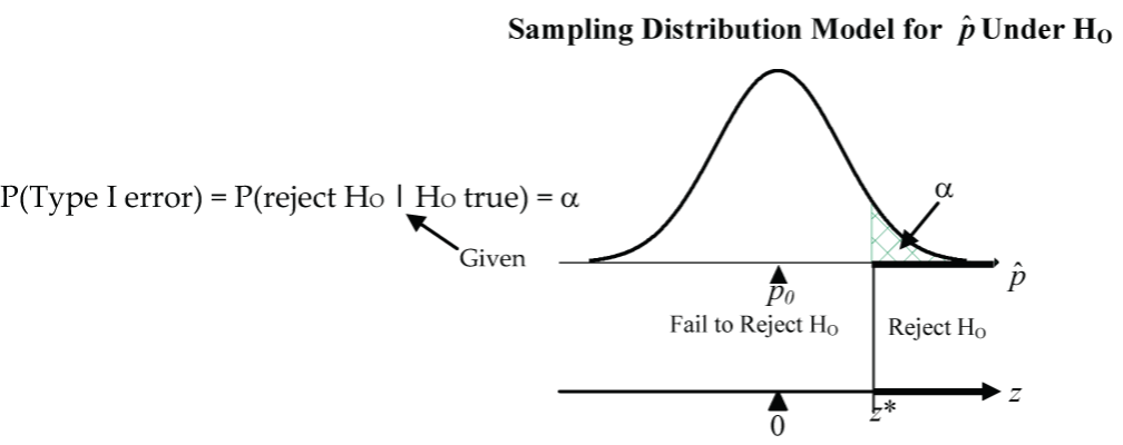
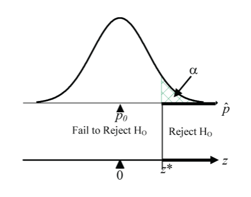
The probability of a Type 2 error is symbolized by  : P(Type 2 error) = P(fail to reject H0 | H0 false) = .
Power of a Statistical Test
Since the significance level is the probability of a Type 1 error, and since we can set the significance level to be as small as we want, why don’t we always set it to be some extremely small number like 0.0001?
Well, there’s a price to be paid! By setting the to be extremely low (pushes z* far to the right), we are demanding extremely convincing evidence that H0 is “guilty,” and this comes at the expense of our test failing to detect moderate departures from H0.
Naturally, we want our statistical test to be “powerful” in detecting departures from the H0 model. Power in the context of a statistical test is the probability that the test will reject H0 when in fact H0 is false.
- Power = P(reject H0 | H0 false)
- = 1 – P(fail to reject H0 | H0 false)
- = 1 – P(Type 2 error)
- = 1 –
So ideally, we want:
- = P(Type 1 error) to be small
- = P(Type 2 error) to be small or, equivalently, Power = 1 – to be large
Thinking back to our drug detection example, the upper pair of normal curves below (Fig. 12) shows the sampling distribution of under the H0 model (p = 0.2) and one possible choice for a HA model (p = 0.3).
How can we reduce both error probabilities and increase the power at the same time?
has reduced variability, which results in normal curves that are more tightly concentrated around their means, which in turn reduces both error probabilities ( and ) and increases the power of the test.
Relationship Between Hypothesis Tests and Confidence Intervals
In a double-blind crossover design, a random sample of 36 patients evaluated two medicated salves. Data Table 2 summarizes the salve preference of each patient.
Patient |
Preferred Salve |
Patient |
Preferred Salve |
| 1 | A | 19 | A |
| 2 | A | 20 | B |
| 3 | B | 21 | A |
| 4 | A | 22 | A |
| 5 | A | 23 | A |
| 6 | A | 24 | B |
| 7 | B | 25 | B |
| 8 | B | 26 | A |
| 9 | A | 27 | A |
| 10 | A | 28 | A |
| 11 | A | 29 | A |
| 12 | A | 30 | A |
| 13 | B | 31 | B |
| 14 | A | 32 | A |
| 15 | B | 33 | A |
| 16 | B | 34 | B |
| 17 | B | 35 | A |
| 18 | A | 36 | A |
- Construct a 90% confidence interval for the proportion of all patients that prefer salve B.
Conditions:
Independence: Reasonable to assume independent trials.
Random: Random sample given.
Success/failure condition: Yes, n = 36(1/3) = 12 ≥ 10 and n = 36(2/3) = 24 ≥ 10
10% condition: Yes, since potential population is very large.
Sample results: 12 out of 36 (1/3) of the patients prefer salve B.
 .
.
90% CI for p: 33.33% ± 12.92%
We are 90% confident that between 20.4% and 46.3% of all patients prefer salve B. - Does the confidence interval in part 1 provide sufficient evidence to conclude that the two salves are not equally preferred at the 0.10 significance level?
H0: p = 0.50 (50%) versus HA: p ≠ 0.50, where p is the proportion of all patients that prefer salve B.
Since the 90% CI in part 1 does not contain the H0 proportion p = 0.50 (50%), we can reject H0 at the 0.10 significance level and conclude that the two salves are not equally preferred.
Generalization
The connection between a general C% confidence interval for p and the corresponding hypothesis test of H0: p = p0 vs. the two-sided HA: p ≠ p0 at the = (100 – C)% significance level is:
- If CI contains p0 then fail to reject H0
- If CI does not contain p0 then reject H0
This equivalency is only approximately true since we use to calculate SE in the CI calculation, but we use to calculate SE when conducting the hypothesis test.
This connection between a confidence interval and a two-sided hypothesis test provides another way to conduct a two-sided hypothesis test. The margin of error in a confidence interval has the form “critical value times standard error.” For example, for a confidence interval for a proportion, the critical value is a z-score from the standard normal distribution corresponding to the specified confidence level (1.6449 in the above example on medical salves).
If the corresponding hypothesis test decision is to reject H0 because the p-value is less than the significance level, then the test statistic must be either greater than the positive critical value (in the upper tail) or less than the negative critical value (in the lower tail). This is often referred to as being in the “rejection region” (less than –1.6449 or greater than 1.6449 in the medical salves example).
In other words, another way to conduct a two-sided hypothesis test is to reject H0 if the test statistic is in the rejection region (either greater than the positive critical value or less than the negative critical value).
For the medical salves example, the test statistic is  . This is in the rejection region since
  , so we reject H0 at the 0.10 significance level.
References
Takeru Kato, Toru Terashima, Takenori Yamashita, Yasuhiko Hatanaka, Akiko Honda, and Yoshihisa Umemura. (2006). Effect of low-repetition jump training on bone mineral density in young women. Journal of Applied Physiology, 100(3), 839-843. https://journals.physiology.org/doi/full/10.1152/japplphysiol.00666.2005
