Supplementary Notes 4.1

Iain Pardoe

Lesson 4.1: Inference for Proportions

Supplementary Notes 4.1

Confidence Interval for a Single Population Proportion

Experimental Situation: One categorical population with an unknown proportion (or percentage) $p$ .

Objective: Based on the results of a random sample of $n$ observations from this population, construct a confidence interval for the unknown proportion $p$ .

Assumptions:

Independence: The individual responses in the sample are independent of each other.
Random: The sample is random.
Success/Failure Condition: $n\hat{p} \ge 10$ and $n\hat{q} \ge 10$ ( $\hat{q} = 1 - \hat{p}$ ).
10% Condition: The sample size $n$ is no more than 10% of the population size.

Confidence Interval Construction: The general form for a confidence interval for a proportion $p$ is $\hat{p} \pm z^* \times \sqrt{\dfrac{\hat{p}\hat{q}}{n}}$ , where $z^*$ is the “critical value” z-score from the standard normal distribution corresponding to the specified confidence level.

Confidence Interval Interpretation: We’re …% confident the population proportion is in the interval … to ….

Hypothesis Test for a Single Population Proportion

Hypotheses
- H₀: p = p₀ versus H_A: p > p₀ (upper-sided alternative)
- H₀: p = p₀ versus H_A: p < p₀ (lower-sided alternative)
- H₀: p = p₀ versus H_A: p ≠ p₀ (two-sided alternative)
Model: Normal model for the sampling distribution of that has a mean of and a SD of , where . Assumptions:
- Independent sample.
- Random sample.
- Success/failure condition: $np_0 \ge 10$ and $nq_0 \ge 10$ .
- 10% condition: The sample size $n$ is no more than 10% of the population size.
Mechanics:
- Upper-sided alternative:
  H₀: p = p₀ versus H_A: p > p₀
  Calculate test statistic: $Z = \dfrac{\hat{p}-p_0}{\sqrt{\dfrac{p_0q_0}{n}}}$

**Figure 1**: Upper-sided proportion test

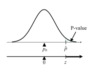
Obtain p-value using R code: 1 - pnorm(Z, mean=0, sd=1)

- Lower-sided alternative:
  H₀: p = p₀ versus H_A: p < p₀
  Calculate test statistic: $Z = \dfrac{\hat{p}-p_0}{\sqrt{\dfrac{p_0q_0}{n}}}$
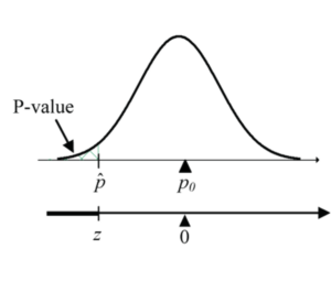
Figure 2: Lower-sided proportion test
- Obtain p-value using R code: pnorm(Z, mean=0, sd=1)
- Two-sided alternative:
  H₀: p = p₀ versus H_A: p ≠ p₀
  Calculate test statistic: $Z = \dfrac{\hat{p}-p_0}{\sqrt{\dfrac{p_0q_0}{n}}}$

**Figure 3**: Two-sided alternative proportion test where p-value is the sum of the two shaded areas.

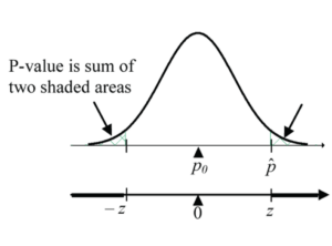
Obtain p-value using R code: 2 * (1 - pnorm(z, mean=0, sd=1))

Conclusion
- If the p-value < the significance level $\alpha$ , reject H₀ in favour of H_A. Conclude that there is sufficient evidence that p > p₀ (upper-sided alternative) or p < p₀ (lower-sided alternative) or p ≠ p₀ (two-sided alternative).
- If the p-value > the significance level $\alpha$ , do not reject H₀. Conclude that there is insufficient evidence that p > p₀ (upper-sided alternative) or p < p₀ (lower-sided alternative) or p ≠ p₀ (two-sided alternative).

Note: Alternatively, in the two-sided case, reject H₀ in favour of H_A if the test statistic is in the rejection region (either greater than the positive critical value or less than the negative critical value). Do not reject H₀ if the test statistic is not in the rejection region (i.e., it is between the negative and positive critical values).

Determining Sample Size for Desired Accuracy and Confidence

Suppose that we wanted to estimate the percentage of adult Vancouverites that support a complete ban on smoking in public places. How large a random sample would we need to make this estimate?

First, we must decide on an acceptable margin of error and confidence level. Suppose that we want our estimate to be within 4% of the population proportion at a 95% confidence level. For proportions, the margin of error is $ME(\hat{p}) = z^* \sqrt{\dfrac{\hat{p}\hat{q}}{n}}$ .

In our application ME = 4% = 0.04 and z* = 1.96 (to achieve 95% confidence).

Now we can find the size of the random sample required by solving for n.

Square each side: $ME^2 = z^{*2} \dfrac{\hat{p}\hat{q}}{n}$
Multiply each side by n: $nME^2 = z^{*2} \hat{p}\hat{q}$
Divide each side by: $ME^2$ : $n = \dfrac{z^{*2} \hat{p}\hat{q}}{ME^2}$
So, in our application: $n = \dfrac{1.96^2 \hat{p}\hat{q}}{0.04^2}$

Problem! We haven’t sampled yet, so we don’t have a value for $\hat{p}$ . What options do we have?

Be cautious and possibly overstate the size of the sample needed by using
$\hat{p}=0.5$ , which gives the largest possible value for the product of $\hat{p}\hat{q}=0.25$ . Convince yourself that all the other choices for $\hat{p}$ give smaller products. For example, $\hat{p}=0.4$ or $\hat{p}=0.6$ gives $\hat{p}\hat{q}=0.24$ and $\hat{p}=0.3$ or $\hat{p}=0.7$ gives $\hat{p}\hat{q}=0.21$ .
If it is available, use an approximation for $\hat{p}$ from a pilot study or prior knowledge.

Do we know anything about the proportion of Vancouverites that support a complete ban on smoking?

If no, use the cautious value $\hat{p}=0.5$ , which gives $n = \dfrac{1.96^2 \hat{p}\hat{q}}{0.04^2} = \dfrac{1.96^2 (0.5)(0.5)}{0.04^2} = 600.25$ . So, we need to randomly sample 601 (always round up these sample size estimates) adult Vancouverites.
If yes, use your prior knowledge to “sharpen the statistical pencil” in your determination of sample size. Likely, the proportion supporting the ban is greater than 50% . Let’s say it is at least 75%. Using $\hat{p}=0.75$ , gives $n = \dfrac{1.96^2 \hat{p}\hat{q}}{0.04^2} = \dfrac{1.96^2 (0.75)(0.25)}{0.04^2} = 450.19$ , this means we need to randomly sample only 451 adult Vancouverites. That’s quite a reduction from the 601. Of course, if we have doubts about our 75% approximation, then we should use the more cautious sample size of 601 that guarantees the desired 4% margin at 95% confidence.

What if we changed the scope of our study to all of Canada? Would we need a much larger sample size?

No! Nothing in the above sample size calculation would change. A random sample of 601 Canadians will estimate the proportion within 4%, “19 times out of 20.” To understand the intuition here, remember the “soup tasting” analogy in Supplementary Notes 1.2 on sample size: A spoonful from a well-mixed small bowl (i.e., Vancouver) will give you just as accurate an assessment of the soup’s flavour as a spoonful from a large bowl (i.e., Canada).

Inference for the Difference of Two Proportions

Is the ginseng-based COLD-FX^® medication effective in reducing the frequency and severity of the common cold? This is an interesting and hotly debated question.

The company that manufactures COLD-FX^® (Bausch Health Companies Inc., formerly CV Technologies Inc.) advertises “Trust the Science” and identifies the results from a number of studies as evidence that their product is effective. The Vancouver Sun columnist David Bains, with the support of Dr. James McCormack and Dr. Peter Loewen at UBC, questioned the results from these studies in a series of articles published on Feb. 25, 2006; Feb. 28, 2006; Mar. 8, 2006; Apr. 12, 2006; June 14, 2006; Oct. 12, 2006; and Nov. 11, 2006. Undoubtedly, this debate will extend into the future as the results from a new multi-million-dollar clinical trial come in. If you think that statistics is dull and without controversy (hard to believe for anyone coming this far in the course!), dig-out these articles and be prepared to change your mind.

We won’t wade into this controversy, but we’ll use one of the results from a study published in the Canadian Medical Association Journal (Predy, 2005) to explore the topic of finding confidence intervals for the difference between two proportions and testing the hypothesis that two proportions are equal.

Efficacy of an Extract of North American Ginseng Containing Poly-Furanosyl-Pyranosyl-Saccharides for Preventing Upper Respiratory Tract Infections: A Randomized Controlled Trial (Predy, 2005)

Used with permission.

Background: Upper respiratory tract infections are a major source of morbidity throughout the world. Extracts of the root of North American ginseng (Panax quinquefolium) have been found to have the potential to modulate both natural and acquired immune responses. We sought to examine the efficacy of an extract of North American ginseng root in preventing colds.

Methods: We conducted a randomized, double-blind, placebo-controlled study at the onset of the influenza season. A total of 323 subjects 18-65 years of age with a history of at least 2 colds in the previous year were recruited from the general population in Edmonton, Alberta. The participants were instructed to take 2 capsules per day of either the North American ginseng extract or a placebo for a period of 4 months. The primary outcome measure was the number of Jackson-verified colds.

Results: Subjects who did not start treatment were excluded from the analysis (23 in the ginseng group and 21 in the placebo group), leaving 130 in the ginseng group and 149 in the placebo group. (…) The proportion of subjects with 2 or more Jackson-verified colds during the 4-month period (10.0% v. 22.8%, 12.8% difference, 95% CI 4.3-21.3) was significantly lower in the ginseng group than in the placebo group ….

Here, two proportions are bring compared: The proportion from the ginseng group getting colds vs. the placebo proportion getting colds. A confidence interval for difference in these two proportions is given as 4.3% to 21.3%. Further, the proportion getting colds for the ginseng group is judged as being significantly lower than the proportion for the placebo group.

How were the results obtained? Please read on!

Confidence Interval for the Difference Between Two Proportions

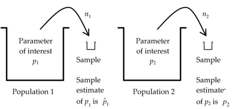
The schematic below illustrates the two-proportion experimental situation as presented in the ginseng study.

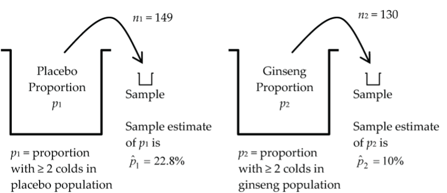
**Figure 4:** Inference for two proportions: placebo proportion and ginseng proportion

Our goal is to develop a confidence interval for the difference, p₁ – p₂.

This CI will have the usual basic form: Sample estimate ± margin of error, which in this case is $\hat{p}_1-\hat{p}_2$ ± margin of error.

This margin of error depends on the sampling distribution of $\hat{p}_1-\hat{p}_2$ . Under certain conditions we know that $\hat{p}_1$ has a normal model with mean $p_1$ and standard deviation $\sqrt{\dfrac{p_1q_1}{n_1}}$ . and $\hat{p}_2$ has a normal model with mean $p_2$ and standard deviation $\sqrt{\dfrac{p_2q_2}{n_2}}$ . It turns out that the difference $\hat{p}_1-\hat{p}_2$ also has a normal model with mean $p_1-p_2$ and standard deviation $\sqrt{\dfrac{p_1q_1}{n_1}+\dfrac{p_2q_2}{n_2}}$ (note there is a plus sign rather than a minus sign in the standard deviation).

Therefore, a confidence interval for the difference, p₁ – p₂, is $\hat{p}_1-\hat{p}_2 \pm z^* \times \sqrt{\dfrac{p_1q_1}{n_1}+\dfrac{p_2q_2}{n_2}}$ . Since $p_1$ and $p_2$ are unknown, we estimate this by $\hat{p}_1-\hat{p}_2 \pm z^* \times \sqrt{\dfrac{\hat{p}_1\hat{q}_1}{n_1}+\dfrac{\hat{p}_2\hat{q}_2}{n_2}}$ .

Now we’re ready to sub in the numbers for the ginseng application to get a 95% CI for the difference in the proportions getting two or more colds for the placebo vs. ginseng groups:

$\hat{p}_1-\hat{p}_2 \pm z^* \times \sqrt{\dfrac{\hat{p}_1\hat{q}_1}{n_1}+\dfrac{\hat{p}_2\hat{q}_2}{n_2}}$
$= 0.228-0.10 \pm 1.96 \times \sqrt{\dfrac{(0.228)(0.772)}{149}+\dfrac{(0.10)(0.90)}{130}}$
$= 0.128 \pm 0.085$
$= 12.8\% \pm 8.5\%$

This gives an interval of 4.3% to 21.3%, as given in the Results section of the Predy (2005) article.

Based on this study, we are 95% confident that the proportion of people getting two or more colds is between 4.3% and 21.3 % higher in the placebo population compared to the ginseng population. Since this interval doesn’t contain zero, it can also be interpreted that the two proportions are statistically significantly different at the 5% significance level, with the ginseng group proportion lower than the placebo group proportion.

Sampling Distribution of the Difference Between Two Proportions

We have already used the normal model for the sampling distribution of $\hat{p}_1-\hat{p}_2$ in the calculation of the confidence interval in the Predy (2005) ginseng study.

What conditions must be satisfied for this normal model to apply?

Basically, we need the same conditions as for the one-proportion case, but now they must apply to each of our two samples, plus we need one more condition: that the two groups are independent. Here is the complete list of necessary conditions:

Independence Between Groups: The two groups that we are comparing are independent of each other. This means that there is no linkage or association between the two groups. This would be the case in a completely randomized experiment where the two groups are formed at random, but it would not be the case if we used twin pairs, for example, to form the two groups.
Independence Within Groups: Within each group, the individual responses are independent of each other.
Random: Each of the two samples is randomly drawn from their respective populations.
Success/Failure Condition: $n_1\hat{p}_1 \ge 10$ , $n_1\hat{q}_1 \ge 10$ , $n_2\hat{p}_2 \ge 10$ , and $n_2\hat{q}_2 \ge 10$ .
10% Condition: Each of the two sample sizes, $n_1$ and $n2$ , is no more than 10% of their respective population sizes.

Under these conditions we have:

$\hat{p}_1-\hat{p}_2$ has a normal model with mean $p_1-p_2$ and standard deviation $\sqrt{\dfrac{p_1q_1}{n_1}+\dfrac{p_2q_2}{n_2}}$ .
A confidence interval for $p_1-p_2$ is $\hat{p}_1-\hat{p}_2 \pm z^* \times \sqrt{\dfrac{\hat{p}_1\hat{q}_1}{n_1}+\dfrac{\hat{p}_2\hat{q}_2}{n_2}}$ .

A Two-Proportion Z-Test

Are the two population proportions equal? We answer this by testing $H_0: p_1=p_2$ or equivalently, $H_0: p_1-p_2=0$ .

What test statistic do we use to judge the weight of the sample evidence against H₀?

If this null hypothesis is true, the difference between the sample proportions, $\hat{p}_1-\hat{p}_2$ , will fluctuate around a mean of zero. If we express the difference, $\hat{p}_1-\hat{p}_2$ , in standardized form by dividing by $\sqrt{\dfrac{p_1q_1}{n_1}+\dfrac{p_2q_2}{n_2}}$ , we’ll be able to judge whether or not $\hat{p}_1-\hat{p}_2$ is unusually far from the mean of zero.

However, how can we calculate $\sqrt{\dfrac{p_1q_1}{n_1}+\dfrac{p_2q_2}{n_2}}$ when we don’t know the values for $p_1$ and $p_2$ ?

We could use $\sqrt{\dfrac{\hat{p}_1\hat{q}_1}{n_1}+\dfrac{\hat{p}_2\hat{q}_2}{n_2}}$ as an approximation. However, there is one more little wrinkle in calculating the two-proportion test statistic for $H_0: p_1=p_2$ .

This null hypothesis says that both unknown population proportions are equal, so rather than two separate estimates it is better to pool them together by taking the average of the two, weighted by their sample sizes, to get one overall estimate of the equal (under the null) unknown proportions: $\hat{p} = \dfrac{n_1\hat{p}_1+n_2\hat{p}_2}{n_1+n_2}$ .

Then calculate the test statistic as $Z = \dfrac{\hat{p}_1-\hat{p}_2}{\sqrt{\dfrac{\hat{p}\hat{q}}{n_1}+\dfrac{\hat{p}\hat{q}}{n_2}}} = \dfrac{\hat{p}_1-\hat{p}_2}{\sqrt{\hat{p}\hat{q}\left(\dfrac{1}{n_1}+\dfrac{1}{n_2}\right)}}$ .

The conditions are the same as listed above for the confidence interval for the difference between two proportions, except the success/failure conditions are now $n_1\hat{p} \ge 10$ , $n_1\hat{q} \ge 10$ , $n_2\hat{p} \ge 10$ , and $n_2\hat{q} \ge 10$ .

Example: Two-Proportion Z-Test

In a study designed to compare the efficacy of “the patch” versus “gum” in helping people quit smoking, 150 smokers were randomly assigned to the patch group (group 1) and 100 smokers to the gum group (group 2).

Do the data (Table 1) provide sufficient evidence to conclude a difference in the percentages quitting smoking with the two methods?

Table 1 Efficacy of Quitting Smoking: Patch or Gum
	Group 1: Patch	Group 2: Gum	Total
Quit smoking	90	50	140
Did not quit	60	50	110
Total	150	100	250

Hypotheses: $H_0: p_1 = p_2$ versus $H_A: p_1 \ne p_2$ .

Pooled proportion: $\hat{p}} = \dfrac{n_1\hat{p}_1+n_2\hat{p}_2}{n_1+n_2} = \dfrac{150(90/150)+100(50/100)}{150+100} = \dfrac{140}{250} = 0.56$ .

Conditions:

Independence Between Groups: Yes, since the two groups were created randomly.
Independence Within Groups: Reasonable to assume.
Random: Unclear how the 250 smokers were selected, but it may have been done randomly.
Success/Failure Condition: $150(0.56) = 84 \ge 10$ , $150(0.44) = 66 \ge 10$ , $100(0.56) = 56 \ge 10$ , and $100(0.44) = 44 \ge 10$ .
10% Condition: Each of the two sample sizes is well below 10% of all smokers using the patch or gum.

Mechanics:

Test statistic, $Z = \dfrac{90/150-50/100}{\sqrt{(0.56)(0.44)\left(\dfrac{1}{150}+\dfrac{1}{100}\right)}} = 1.5605$ .
P-value = 2 * (1 - pnorm(1.5605, mean=0, sd=1)) ≈ 0.1186. (Note the upper-tail area is doubled because of the two-sided alternative hypothesis.)

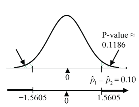
Smoking example — ***Figure 6:*** *Two-sided alternative proportion test: The p-value is the sum of two shaded areas.*

So, if the rates quitting smoking really are the same for the two groups (H₀ true), there is about a 11.86% chance that we would observe sample proportions that differ by 10% (60% – 50%) or more. This is not unusual enough to reject H₀ at a 5% significance level.

Conclusion:

The sample evidence is not strong enough for us to conclude a difference in the percentages quitting smoking with the two methods.

Alternatively, reject H₀ in favour of H_A if the test statistic is in the rejection region (either greater than the positive critical value or less than the negative critical value). Do not reject H₀ if the test statistic is not in the rejection region (i.e., it is between the negative and positive critical values). The critical value in the smoking example is 1.9600, the 97.5^th percentile of the standard normal distribution. Since the test statistic, $Z=1.5605$ is between –1.9600 and 1.9600, it is not in the rejection region, so we do not reject H₀.

References

Predy, G. N. (2005). Efficacy Of An Extract Of North American Ginseng Containing Poly-furanosyl-pyranosyl-saccharides For Preventing Upper Respiratory Tract Infections: A Randomized Controlled Trial. Canadian Medical Association Journal, 173(9), 1043-1048. https://doi.org/10.1503/cmaj.1041470

License

Icon for the Creative Commons Attribution-NonCommercial-ShareAlike 4.0 International License

Introduction to Probability and Statistics Copyright © 2023 by Thompson Rivers University is licensed under a Creative Commons Attribution-NonCommercial-ShareAlike 4.0 International License, except where otherwise noted.