Supplementary Notes 4.2

Iain Pardoe

Lesson 4.2: Testing Goodness of Fit in One-way Tables

Supplementary Notes 4.2

Chi-Square Models

The inference problems we have considered so far have involved proportions, which we can think of as summarizing a categorical variable with two categories; for example, supporting/opposing an aquarium expansion, or quitting/failing to quit smoking. Here, we will consider inference involving a categorical variable with more than two categories.

Given data separated into different categories, we will test whether an observed distribution is consistent with what we expected. We want to know whether observed differences among counts in different categories are large enough to be significant. To do this, we need a new family of models called chi-square, which in symbols is written χ² (“chi” is another Greek symbol, like alpha, $\alpha$ , and beta, $\beta$ ).

Chi-square models also allow us to decide whether we think two categorical variables are independent, which we’ll consider in Lesson 4.3. Finally, we will have a tool that will enable us to answer a question we asked in Supplementary Notes 1.4 about the independence of two categorical variables (remember the example on smoking status and blood group?). Chi-square models are different from the normal model we’ve used in previous analyses. In particular, chi-square models only take positive values and are skewed to the right. Whereas we need two parameters (the mean and the standard deviation) to specify a normal model, the only parameter needed to specify a chi-square distribution is the degrees of freedom (denoted by df).

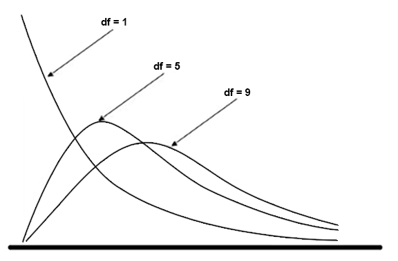
**Figure 1**: Density functions for chi-square distributions with different degrees of freedom (df)

The degrees of freedom of a chi-square model increases as the number of categories increases.

Goodness-of-Fit Tests

Suppose you roll a six-sided die 600 times, and you wish to test if the die is fair. You obtain the following counts (Table 1) of the outcomes one to six:

Table 1 Outcomes of 600 Die Rolls
Die Outcome	1	2	3	4	5	6
Frequency	96	94	90	89	114	117

Hypotheses

The null hypothesis of this goodness-of-fit test is that the probability model is correct, and that all faces of the die are equally likely to occur. You are testing whether the observed frequencies are consistent with the model or vary so much from a perfect 1:1:1:1:1:1 ratio to cast doubt on the fairness of the die.

H₀: The die is fair (all outcomes are equally likely).
H_A: The die is not fair.

If the die is fair, how many of each of the outcomes (one to six) would you expect?

Since you rolled the die 600 times, you would expect each outcome to occur 100 times. These are called the expected counts (Exp). The frequencies actually obtained are called the observed counts (Obs). Note that while observed counts must be whole numbers, expected counts need not be.

Test Statistic

The test statistic for the chi-square test is $\chi^2 = \sum \dfrac{(Obs-Exp)^2}{Exp}$ .

It is found by adding-up the sum of squares of the deviations between the observed and expected counts divided by the expected counts. The degrees of freedom for this goodness-of-fit test is the number of categories minus one.

Assumptions and Conditions

When the conditions below are met, $\chi^2 = \sum \dfrac{(Obs-Exp)^2}{Exp}$ follows a chi-square model with k – 1 df, where k is the number of categories.

Counted Data Condition: The data must be counts (frequencies) for the categories of a categorical variable.
Independence: The counts in the cells should be independent of each other.
Random: The sample is random.
Expected Cell Frequency Condition: All expected cell frequencies must be at least five. If a small number of cells have expected counts slightly less than five, you can proceed with caution. However, if it makes sense to do so, it is better to combine cells with expected counts less than five. There is no similar cell frequency condition for the observed counts.
10% Condition: The sample size is no more than 10% of the population size.

When performing a chi-square goodness-of-fit test, it is important to check the above conditions by showing all the expected counts, and not just a claim that they are satisfied without showing any evidence.

Are chi-square tests one-tailed or two-tailed?

As mentioned earlier, chi-square models take-on only non-negative values and are skewed to the right. Thus, the tests are always one-sided with the rejection region in the upper tail.

Mechanics

We will calculate the chi-square test statistic value with the help of Table 2.

Table 2 Chi-Square Statistic Values for Die Rolls
Die Outcome	Observed	Expected	Residual (Obs – Exp)	(Obs – Exp)²	Component (Obs – Exp)² / Exp
1	96	100	-4	16	0.16
2	94	100	-6	36	0.36
3	90	100	-10	100	1
4	89	100	-11	121	1.21
5	114	100	14	196	1.96
6	117	100	17	289	2.89
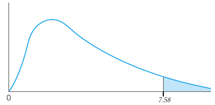
					Sum = 7.58

Although it helps to keep the calculations organized in a table, you do not need to use one to calculate the χ² test statistic value since we can also calculate it as:

$\chi^2 = \dfrac{(96-100)^2}{100} + \dfrac{(94-100)^2}{100} + \dfrac{(90-100)^2}{100} +$ $\dfrac{(89-100)^2}{100} + \dfrac{(114-100)^2}{100} + \dfrac{(117-100)^2}{100} = 7.58$ .

So χ² = 7.58 and df = 6 − 1 = 5, as there are six categories.

P-value calculation: 1 - pchisq(7.58, df=5) ≈ 0.181.

Conclusion

With a p-value = 0.181 (shaded area in Figure 2), which is greater than a significance level, $\alpha$ , of 0.05, there is insufficient evidence to reject the null hypothesis. The data support the claim that the die is fair.

chi-square goodness of fit test — **Figure 2:** Chi-square with df = 5

Alternatively, reject H₀ in favour of H_A if the test statistic is in the rejection region (greater than the critical value). Do not reject H₀ if the test statistic is not in the rejection region (less than the critical value). The critical value in the six-sided die example is 11.0705, the 95^th percentile of the chi-square distribution with five degrees of freedom. Since the test statistic, χ² = 7.58 is less than 11.0705, it is not in the rejection region, so we do not reject H₀.

License

Icon for the Creative Commons Attribution-NonCommercial-ShareAlike 4.0 International License

Introduction to Probability and Statistics Copyright © 2023 by Thompson Rivers University is licensed under a Creative Commons Attribution-NonCommercial-ShareAlike 4.0 International License, except where otherwise noted.